17) Reconstructions and slope/flux limiters#
Notes on unstructured meshing workflow
Finite volume methods for hyperbolic conservation laws
Riemann solvers for scalar equations
Shocks and the Rankine-Hugoniot condition
Rarefactions and entropy solutions
Today:
Godunov’s Theorem
Slope reconstruction and limiting
2.1 Common limiters in the FV literatureIntroduction on hyperbolic systems
3.1 Example: Isentropic gas dynamics
using LinearAlgebra
using Plots
default(linewidth=3)
using LaTeXStrings

# utility functions for Runge-Kutta ODE time-steppers
struct RKTable
    A::Matrix
    b::Vector
    c::Vector
    function RKTable(A, b)
        s = length(b)
        A = reshape(A, s, s)
        c = vec(sum(A, dims=2))
        new(A, b, c)
    end
end

rk4 = RKTable([0 0 0 0; .5 0 0 0; 0 .5 0 0; 0 0 1 0], [1, 2, 2, 1] / 6)

function ode_rk_explicit(f, u0; tfinal=1., h=0.1, table=rk4)
    u = copy(u0)
    t = 0.
    n, s = length(u), length(table.c)
    fY = zeros(n, s)
    thist = [t]
    uhist = [u0]
    while t < tfinal
        tnext = min(t+h, tfinal)
        h = tnext - t
        for i in 1:s
            ti = t + h * table.c[i]
            Yi = u + h * sum(fY[:,1:i-1] * table.A[i,1:i-1], dims=2)
            fY[:,i] = f(ti, Yi)
        end
        u += h * fY * table.b
        t = tnext
        push!(thist, t)
        push!(uhist, u)
    end
    thist, hcat(uhist...)
end

# utility functions for Riemann problems and FV
function testfunc(x)
    max(1 - 4*abs.(x+2/3),
        abs.(x) .< .2,
        (2*abs.(x-2/3) .< .5) * cospi(2*(x-2/3)).^2
    )
end

flux_advection(u) = u
flux_burgers(u) = u^2/2
flux_traffic(u) = u * (1 - u)

riemann_advection(uL, uR) = 1*uL # velocity is +1

function fv_solve1(riemann, u_init, n, tfinal=1)
    h = 2 / n
    x = LinRange(-1+h/2, 1-h/2, n) # cell midpoints (centroids)
    idxL = 1 .+ (n-1:2*n-2) .% n
    idxR = 1 .+ (n+1:2*n) .% n
    function rhs(t, u)
        fluxL = riemann(u[idxL], u)
        fluxR = riemann(u, u[idxR])
        (fluxL - fluxR) / h
    end
    thist, uhist = ode_rk_explicit(rhs, u_init.(x), h=h, tfinal=tfinal)
    x, thist, uhist
end

function riemann_burgers(uL, uR)
    flux = zero(uL)
    for i in 1:length(flux)
        fL = flux_burgers(uL[i])
        fR = flux_burgers(uR[i])
        flux[i] = if uL[i] > uR[i] # shock
            max(fL, fR)
        elseif uL[i] > 0 # rarefaction all to the right
            fL
        elseif uR[i] < 0 # rarefaction all to the left
            fR
        else
            0
        end
    end
    flux
end

function riemann_traffic(uL, uR)
    flux = zero(uL)
    for i in 1:length(flux)
        fL = flux_traffic(uL[i])
        fR = flux_traffic(uR[i])
        flux[i] = if uL[i] < uR[i] # shock
            min(fL, fR)
        elseif uL[i] < .5 # rarefaction all to the right
            fL
        elseif uR[i] > .5 # rarefaction all to the left
            fR
        else
            flux_traffic(.5)
        end
    end
    flux
end
riemann_traffic (generic function with 1 method)
Recall from last lecture that the Burger’s equation has a nonlinear flux, so we found shock waves and rarefaction waves.
init_func(x) = testfunc(x) - .5
x, thist, uhist = fv_solve1(riemann_burgers, init_func, 200, 1)
plot(x, uhist[:,1:20:end], legend=:none, xlabel = L"x", ylabel = L"u")

Recap#
Some examples seen so far:
Burgers#
flux \(u^2/2\) has speed \(u\)
negative values make sense
satisfies a maximum principle
Traffic#
flux \(u - u^2\) has speed \(1 - 2u\)
state must satisfy \(u \in [0, 1]\)
1. Godunov’s Theorem (1954)#
Linear numerical methods
For our purposes, monotonicity is equivalent to positivity preservation,
Discontinuities#
A numerical method for representing a discontinuous function on a stationary grid can be no better than first order accurate in the \(L^1\) norm,
In light of these two observations, we may still ask for numerical methods that are more than first order accurate for smooth solutions, but those methods must be nonlinear.
2. Slope reconstruction and limiting#
For many finite-difference or finite-volume computations with discontinuous solutions limiters are a necessary evil. NASA’s Technical Report by Berger, Aftosmis, and Murman (2005)
One method for constructing higher order methods is to use the state in neighboring elements to perform a conservative reconstruction of a piecewise polynomial, then compute numerical fluxes by solving Riemann problems at the interfaces.
If \(x_i\) is the center of cell \(i\) and \(g_i\) is the reconstructed gradient inside cell \(i\), our reconstructed solution \(\tilde u_i(x)\) is
We would like this reconstruction to be monotone in the sense that
Question#
Is the symmetric centered difference slope
Flux limiting#
We will determine gradients by “limiting” the above slope using a nonlinear function that reduces to 1 when the solution is smooth.
There are many ways to express flux/slope limiters and our discussion here roughly follows this NASA’s Technical Report by Berger, Aftosmis, and Murman (2005).
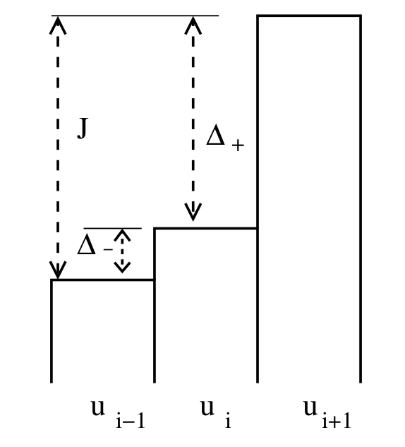
The figure above depicts cell averages corresponding to the limiters. When \(u_i\) is exactly in the middle, the data is linear, and
and the limiter is \(1\). The undivided differences are \(\Delta_{-} = u_i − u_{i−1}\) , and \(\Delta_+ = u_{i+1} − u_i\). \(J\) is the total jump \(u_{i+1} − u_{i−1}\). This introduced variable \(f\) varies between \(0\) and \(1\) as the solution varies from \(u_{i-1}\) to \(u_{i+1}\). It has the purpose of more clearly relating the location of \(u_i\) to the limiter value.
Flux-corrected Transport (FCT) Zalesak 1979#
Zalesak proposed a linear combination of low-order (think 1st order) and high-order (think 3rd-order) upwinding. For example, one can write a second-order scheme as a first-order scheme plus a limited anti-diffusive flux, shown here for a linear advection/transport equation
Zalesak’s proposed modified scheme is
where the anti-diffusive flux is \(F_{i+1/2} = \frac{\lambda}{2} (1-\lambda) (u_{i+1} -u_i)\) that has the effect of sharpening up a regular upwind approximation that would be overly diffusive. Here \(\lambda = a \frac{\Delta t}{\Delta x}\) and \(\phi\)’s are the flux limiters. These have the role of changing the magnitude of the correction actually used, depending on how the solution is behaving. Ideally we would like to apply the limiters in such a way that the discontinuous portion of the solution remains nonoscillatory while the smooth portion remains accurate. To do so we must use the characteristic structure of the solution.
Observations:
We note that in the above, when \(\phi_i = 0\), we recover the low-order (1st order) upwind scheme, and when \(\phi_i = 1\) we have a higher-order method.
The first-order upwind method is Total Variation Diminishing (TVD) for the advection equation. Meaning, the upwind method may smear solutions but cannot introduce oscillations.
If a method is TVD, then in particular data that is initially monotone will remain monotone in all future time steps.
Hence if we discretize a single propagating discontinuity, with a TVD method the discontinuity may become smeared in future time steps but cannot become oscillatory.
All TVD methods are also monotonicity-preserving.
We will express a slope limiter in terms of the ratio of backward to forward differences in the solution
where we have followed the notation used in Sweby, High Resolution Schemes Using Flux Limiters for Hyperbolic Conservation Laws (1984) (which is the inverse of the \(R_i\) used in the Berger, Aftosmis, and Murman (2005) technical report):
Sweby (1984) derived the well-known result
For second order accuracy away from extrema, the flux limiter must satisfy \(\psi(1) = 1\).
In other words, the method should not do any limiting when the solution is a linear function.
For all flux limiters, a negative value of \(R\) indicates an extremum in the solution at cell \(i\), and all set \(\psi(R \leq 0) = 0\). For \(R \geq 0\), the most common limiters are given below.
Also, \(\psi\) must be symmetric
This symmetry is not immediately apparent. We will rewrite these flux limiters as slope limiters in a more transparently symmetric form.
Slope limiters#
Spekreijse (1987) showed the equivalence of flux limiting with slope limiting, which is more natural for Finite Volume schemes in REP form: Reconstruct the solution from its cell averages, Evolve the reconstructed solution from time \(t^n\) to \(t^{n+1}\) , and Project the solution back onto the grid to update the integral cell averages at the new time.
We use the linear advection/transport equation again as an exemplar hyperbolic PDE. We compute states in the flux form for linear advection, using the one-sided differences. Computing the states at the cell interfaces gives
where \(u^L_{i+\frac12}\) is the left state at the right edge and \(u^R_{i-\frac12}\) is the right state at the left edge.
Requiring that this be equivalent to reconstructing with a single limited gradient in cell \(i\), and using the central difference
gives:
Thus, we get the relationship between the flux limiter \(\psi\) and the slope limiter \(\phi\)
Slope limiters make the reconstruction step easy, and, again, we write the reconstructed function \(\tilde u_i(x)\) as
where, again, \(u_i\) is the cell average.
Now, the slope limiter \(\phi\) satisfies this form of the symmetry condition
\(\phi(r) \equiv 1, \forall r\) gives the Lax–Wendroff method (which makes the reconstruction exact for a linear profile).
\(\phi(r) \equiv 0, \forall r\) gives regular upwind.
More generally we might want to devise a limiter function \(\phi\) that has values near \(1\) for \( r \approx 1\), but that reduces (or perhaps increases - depending on the sign of the propagation speed) the slope where the data is not smooth.
The main idea is again to use the centered finite difference scheme for the slope, \( \hat g_i\), and multiply it by a nonlinear factor \(\phi (r_i)\) which detects whether the local data are smooth and monotone.
If the solution is locally linear, then we have the approximation
If \(r_i \leq 0\), then \(u_i\) is not between its neighbors, which is a warning sign for an extremum or non-monotone data, so the limiter cuts the slope down or all the way to zero.
This is the mechanism that avoids Gibbs-like oscillations near shocks.
With the aid of the auxiliary independent variable
the following figure shows the different slope limiters \(\phi(f)\) as a function of the independent variable \(f\). As the solution \(u_i\) varies from \(u_{i-1} to \)u_{i+1}\( , \)f\( varies between \)0\( and \)1$.
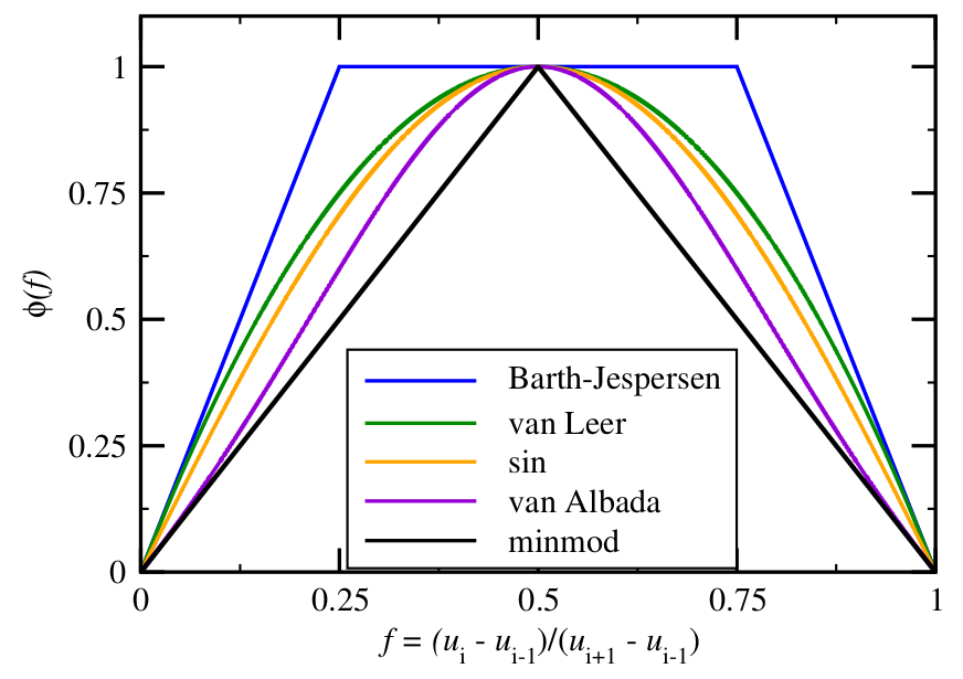
All of these limiters are second order accurate and total variation diminishing (TVD); those that fall below “minmod” are not second order accurate and those that are above Barth-Jesperson are not second order accurate, not TVD, or produce artifacts.
To plot the limiters as a function of \(f\), we define \(w(f) = \phi(R(f))\) and use the symmetry property (38) to get
showing that on uniform grids the graph should be symmetric about \(f = \frac{1}{2}\). On uniform meshes \(f = \frac12\) corresponds to linear data for \(u\).
It is the neighbor of \(u_i\) with the larger jump, either \(u_{i+1}\) or \(u_{i-1}\), that causes the limiting of \(u_i\)’s slope, since it is this jump that would cause the overshoot at the opposite neighbor’s face.
2.1 Common limiters in the FV literature#
Referring to the names used in the code below, we have:
limit_zero#
so the reconstructed slope is always zero:
This gives a piecewise constant reconstruction in each cell, which is just the first-order upwind Godunov method. It is the most diffusive limiter.
limit_none#
so the reconstructed slope is:
which is the unlimited centered finite difference slope. It is second-order in smooth regions but can create under/overshoots.
limit_minmod#
This behaves like
This creates a triangular shape with peak value \(1\) at \(f=1/2\). It is a conservative, fairly dissipative limiter: it allows a slope only when the cell average \(u_i\) lies between its two neighbors, and even then it trims the slope aggressively as you move away from the linear case \(f=1/2\).
limit_sin#
smoother than the previous one with same extrema behavior.
limit_vl#
Similar to the previous one, quadratic shape (parabola) transition instead of a trigonometric one.
limit_bj#
This grows linearly from zero, then plateaus at 1 through a broad middle region, then decreases linearly back to zero as \(f \to 1\). It is more permissive than minmod: if the solution looks reasonably smooth and monotone, it keeps the full centered slope over a larger range of \(f\)-values.
limit_zero(f) = 0 # piecewise constant in each cell
limit_none(f) = 1 # no limiter, centered diff
limit_minmod(f) = max(min(2*f, 2*(1-f)), 0)
limit_sin(f) = (0 < f && f < 1) * sinpi(f)
limit_vl(f) = max(4*f*(1-f), 0)
limit_bj(f) = max(0, min(1, 4*f, 4*(1-f)))
limiters = [limit_zero limit_none limit_minmod limit_sin limit_vl limit_bj];
plot(limiters, label=limiters, xlims=(-.1, 1.1), xlabel = L"f", ylabel = L"\phi(f)")

A FV solver with flux/slope limiter#
function fv_solve2(riemann, u_init, n, tfinal=1, limit=limit_sin)
    h = 2 / n # 1D domain [-1,1]
    x = LinRange(-1+h/2, 1-h/2, n) # cell midpoints (centroids)
    idxL = 1 .+ (n-1:2*n-2) .% n
    idxR = 1 .+ (n+1:2*n) .% n
    function rhs(t, u)
        jump = u[idxR] - u[idxL]
        r = (u - u[idxL]) ./ jump
        r[isnan.(r)] .= 0
        g = limit.(r) .* jump / 2h
        fluxL = riemann(u[idxL] + g[idxL]*h/2, u - g*h/2)
        fluxR = fluxL[idxR]
        (fluxL - fluxR) / h
    end
    thist, uhist = ode_rk_explicit(
        rhs, u_init.(x), h=h, tfinal=tfinal)
    x, thist, uhist
end
fv_solve2 (generic function with 3 methods)
x, thist, uhist = fv_solve2(riemann_advection, testfunc, 200, 10,
    limit_sin)
plot(x, uhist[:,1:400:end], legend=:none, xlabel = L"x", ylabel = L"u")

3. Introduction on hyperbolic systems#
Systems of the form
It would be too good if we could safely reconstruct each component of the flux in the same way.
But the system has waves traveling at different speeds. So we need to be more careful with reconstructions.
3.1 Example: Isentropic gas dynamics#
Variable |
meaning |
|---|---|
\(\rho\) |
density |
\(u\) |
velocity |
\(\rho u\) |
momentum |
\(p\) |
pressure |
Isentrtropic equation of state (pressure depends only on density) \(p(\rho) = C \rho^\gamma\) with \(\gamma = 1.4\) (typical air).
“isothermal” gas dynamics: \(p(\rho) = c^2 \rho\), wave speed \(c\).
Compute the needed \(\rho u^2\) as \( \rho u^2 = \frac{(\rho u)^2}{\rho} .\)
The flux Jacobian is
Smooth wave structure#
For perturbations of a constant state, systems of equations produce multiple waves with speeds equal to the eigenvalues of the flux Jacobian,