14) FEM Assembly#
Last time:
Introduction to the Finite Element Method
Variational formulations
Galerkin Spectral Element Method (SEM): \(L^2\) projection
Today:
Linear Finite Elements
Galerkin method for 1D Poisson equation
Abstractions
Efficiency of matrix-free representations
1. Linear Finite Elements#
The domain \(\Omega = [0,1]\) is discretized with elements (subintervals \(\Omega_h\))
such that \(x_i = i h \), \(i=0,1,\ldots, n\), where
is the length of the subinterval \((x_{i-1}, x_i)\), \(i=1, 2, \ldots, n\).
Linear (Hat) Basis Functions#
Nodal Property#
where \(\delta_{ij}\) denotes the Kronecker delta. This just says that \(\phi_i(x)\) has zeros at all the \(x_j\)’s (with \(j \neq i\)) except \(x_i\), where it is identically equal to \(1\).
Compact support#
Derivatives#
Uniform Mesh Case#
When a mesh is partitioned in uniform (all identically equal) elements, we have that \(h_i = h\) and therefore, we can rewrite
using Plots
using LaTeXStrings
default(linewidth=4, legendfontsize=12)

# Piecewise linear hat function centered at node xc,
# with left neighbor xl and right neighbor xr
function hat(x, xl, xc, xr)
    if x < xl || x > xr
        0.0
    elseif x <= xc
        (x - xl) / (xc - xl)
    else
        (xr - x) / (xr - xc)
    end
end

xim1 = -1.0
xi   =  0.0
xip1 =  1.0

x = range(xim1 - 0.5, xip1 + 0.5, length=500)
phi_i = [hat(xx, xim1, xi, xip1) for xx in x]

plot(x, phi_i,
    lw=3,
    label=L"\phi_i(x)",
    xticks=([xim1, xi, xip1], [L"x_{i-1}", L"x_i", L"x_{i+1}"]),
    yticks=([0, 1], ["0", "1"]),
    ylims=(-0.05, 1.1),
    framestyle=:origin
)

scatter!([xim1, xi, xip1], [0, 1, 0], label="")

# Example node locations
xim2 = -2.0
xim1 = -1.0
xi   =  0.0
xip1 =  1.0
xip2 =  2.0

# Plot grid
x = range(xim2, xip2, length=1000)

# Three hat functions
phi_im1 = [hat(xx, xim2, xim1, xi)   for xx in x]
phi_i   = [hat(xx, xim1, xi,   xip1) for xx in x]
phi_ip1 = [hat(xx, xi,   xip1, xip2) for xx in x]

# Base plot
plot(x, phi_im1,
    lw=3,
    label=L"\phi_{i-1}(x)",
    xlabel=L"x",
    ylabel="",
    legend=:top,
    ylims=(-0.05, 1.2),
    xlims=(xim2 - 0.4, xip2 + 0.5),
    xticks=([xim2, xim1, xi, xip1, xip2],
            [L"x_{i-2}", L"x_{i-1}", L"x_i", L"x_{i+1}", L"x_{i+2}"]),
    yticks=[],
    framestyle=:origin
)

plot!(x, phi_i,   lw=3, label=L"\phi_i(x)")
plot!(x, phi_ip1, lw=3, label=L"\phi_{i+1}(x)")

# Mark the nodes
scatter!([xim2, xim1, xi, xip1, xip2], zeros(5),
    label="",
    markersize=5
)

# Optional vertical guide lines at the peaks
plot!([xim1, xim1], [0, 1], lw=1, ls=:dash, color=:black, label="")
plot!([xi,   xi],   [0, 1], lw=1, ls=:dash, color=:black, label="")
plot!([xip1, xip1], [0, 1], lw=1, ls=:dash, color=:black, label="", legend =:topright)

2. Galerkin method for 1D Poisson equation#
For the 1D two-point BVP for the Poisson equation:
We have seen that we start by constructing a weak form or variational formulation of the problem
Step 1: Multiply both sides of the PDE by a test function \(v(x)\) with compact support (i.e., \( v(0)=0, \; v(1) = 0 \)).
Step 2: Integrate both sides of the equation across the domain \(\Omega = [0,1]\) and apply integrations by parts. On the left-hand-side we have:
We note that the boundary term vanishes because \(v\) has compact support.
Hence the weak form of the PDE is:
and we want to find \(u\) such as this holds \(\forall v\).
Step 3: Construct the set of linear (hat) basis function as above
Step 4: Expand all functions in terms of basis functions, such as
where the coefficients \(\{u_j\}\) are the unknown nodal values to be determined and the \(\{v_j\}\) are arbitrary (since the weak form has to hold \(\forall v\)).
On assuming the hat basis functions, obviously \(u_h(x)\) is also a piecewise linear function, although this is not usually the case for the true solution \(u(x)\).
In general, we have the weak form
When we substitute the expansions of \(u\) and \(v\) in terms of basis functions, we get
the integral are linears, so we can bring the \(v_i\) coefficients outside of the integral sign
Then the equation becomes:
Since the coefficients \(v_i\) are arbitrary, the only way this equation holds for all \(v\) is:
For our specific case, we are finally ready derive a linear system of equations for the coefficients by substituting the approximate solution \(u_h(x)\) for the exact solution \(u(x)\) in the weak form (17)
Hence,
Because the weak form has to hold \(\forall v\) (hence, the \(v_i\) are arbitrary), we have that the expansion of the test function \(v\) in the equation above leads to the following system of equations in which the \(v_i\) coefficients do not appear (given the argument shown above for the general weak form)
Or in matrix form:
Where we have used the bilinear form
and the inner product
The matrix problem above can be written more compactly as
where the matrix \(K\) is called the Stiffness Matrix.
Therefore, for this case we get the matrix
The right-hand side can be explicitly written as
where we have used the simple trapezoidal rule for the \(L^2\) inner product integral.
Hence, we can rewrite our matrix problem as
Step 5: Solve the linear system of equations for the coefficients \( \{u_j\}\) and hence obtain the approximate solution
\[ u_h(\mathbf x) = \sum_{j=1}^n u_j \, \phi_j(\mathbf x) \]
We note that the role of \(v\) as a test function is to be used to extract equations for \(u\), but it is not an unknown.
Observations#
Does the matrix in (18) look familiar??
We note that for solving \(-u'' = f(x)\), \(u(0) = u(1) = 0\), the matrix form of the \(P^1\) linear Finite Element Method with trapezoidal quadrature is precisely the second order centered Finite Difference Scheme.
3. Abstractions#
Tip
Some useful resources for FEM/SEM are:
libCEED documentation, especially the Mathematical Framework and Examples sections
The Dolfinx/FeniCS Tutorial, especially their Fundamentals section
The deal.ii project has extensive documentation on FEM
Ferrite.jl, a Julia library for FEM that has a nice documentation, especially the Topic guides and Tutorials sections.
In general, In the FEM/SEM formulations, we always try to keep the order of derivatives of \(u\) and \(v\) as small as possible. We reach a general form, where we can express as \(f_0\) all terms in the weak form that multiply the test function \(v\) and \(f_1\) all terms that multiply its gradient \(\nabla v\):
General form:
Where \(f_0\) is the contribution given by everything that multiplies the test function \(v\) and \(f_1\) is the contribution given by everything that multiplies the gradient of the test function \(\nabla v\).
Many FEM/SEM libraries (like libCEED) discretize this as
libCEED’s operator decomposition is summarized in the following graphic.

Isoparametric mapping#
Given the reference space coordinates \(X \in \hat K \subset \mathbb{R}^n\) and physical space coordinates \(x(X)\), an integral on the physical element \(K\) can be written
Notation |
Meaning |
|---|---|
\(x\) |
physical coordinates |
\(X\) |
reference coordinates |
\(\mathcal E_e\) |
restriction from global vector to element \(e\) |
\(B\) |
values of nodal basis functions at quadrature ponits on reference element |
\(D\) |
gradients of nodal basis functions at quadrature points on reference element |
\(W\) |
diagonal matrix of quadrature weights on reference element |
\(\frac{\partial x}{\partial X} = D \mathcal E_e x \) |
gradient of physical coordinates with respect to reference coordinates |
\(\left\lvert \frac{\partial x}{\partial X}\right\rvert\) |
determinant of coordinate transformation at each quadrature point |
\(\frac{\partial X}{\partial x} = \left(\frac{\partial x}{\partial X}\right)^{-1}\) |
derivative of reference coordinates with respect to physical coordinates |
Finite element mesh and restriction#
using LinearAlgebra
using SparseArrays
using FastGaussQuadrature

function my_spy(A)
    cmax = norm(vec(A), Inf)
    s = max(1, ceil(120 / size(A, 1)))
    spy(A, marker=(:square, s), c=:diverging_rainbow_bgymr_45_85_c67_n256, clims=(-cmax, cmax))
end

function vander_legendre_deriv(x, k=nothing)
    if isnothing(k)
        k = length(x) # Square by default
    end
    m = length(x)
    Q = ones(m, k)
    dQ = zeros(m, k)
    Q[:, 2] = x
    dQ[:, 2] .= 1
    for n in 1:k-2
        Q[:, n+2] = ((2*n + 1) * x .* Q[:, n+1] - n * Q[:, n]) / (n + 1)
        dQ[:, n+2] = (2*n + 1) * Q[:,n+1] + dQ[:,n]
    end
    Q, dQ
end

# build the reference-element basis functions evaluated at quadrature points
function febasis(P, Q)
    x, _ = gausslobatto(P)
    q, w = gausslegendre(Q)
    Pk, _ = vander_legendre_deriv(x)
    Bp, Dp = vander_legendre_deriv(q, P)
    B = Bp / Pk
    D = Dp / Pk
    x, q, w, B, D
end

function L2_galerkin(P, Q, f)
    x, q, w, B, _ = febasis(P, Q)
    A = B' * diagm(w) * B
    rhs = B' * diagm(w) * f.(q)
    u = A \ rhs
    x, u
end
L2_galerkin (generic function with 1 method)
# 1D finite-element mesh topology and local-to-global connectivity operator used later in assembly
function fe1_mesh(P, nelem)
    x = LinRange(-1, 1, nelem+1)
    rows = Int[]
    cols = Int[]
    for i in 1:nelem
        append!(rows, (i-1)*P+1:i*P)
        append!(cols, (i-1)*(P-1)+1:i*(P-1)+1)
    end
    x, sparse(cols, rows, ones(nelem*P))'
end
P, nelem = 4, 3
x, E = fe1_mesh(P, nelem)
E
12×10 Adjoint{Float64, SparseMatrixCSC{Float64, Int64}} with 12 stored entries:
 1.0   ⋅    ⋅    ⋅    ⋅    ⋅    ⋅    ⋅    ⋅    ⋅
  ⋅   1.0   ⋅    ⋅    ⋅    ⋅    ⋅    ⋅    ⋅    ⋅
  ⋅    ⋅   1.0   ⋅    ⋅    ⋅    ⋅    ⋅    ⋅    ⋅
  ⋅    ⋅    ⋅   1.0   ⋅    ⋅    ⋅    ⋅    ⋅    ⋅
  ⋅    ⋅    ⋅   1.0   ⋅    ⋅    ⋅    ⋅    ⋅    ⋅
  ⋅    ⋅    ⋅    ⋅   1.0   ⋅    ⋅    ⋅    ⋅    ⋅
  ⋅    ⋅    ⋅    ⋅    ⋅   1.0   ⋅    ⋅    ⋅    ⋅
  ⋅    ⋅    ⋅    ⋅    ⋅    ⋅   1.0   ⋅    ⋅    ⋅
  ⋅    ⋅    ⋅    ⋅    ⋅    ⋅   1.0   ⋅    ⋅    ⋅
  ⋅    ⋅    ⋅    ⋅    ⋅    ⋅    ⋅   1.0   ⋅    ⋅
  ⋅    ⋅    ⋅    ⋅    ⋅    ⋅    ⋅    ⋅   1.0   ⋅
  ⋅    ⋅    ⋅    ⋅    ⋅    ⋅    ⋅    ⋅    ⋅   1.0
# build global coordinates for all DOFs from element boundary points
function xnodal(x, P)
    xn = Float64[]
    xref, _ = gausslobatto(P)
    for i in 1:length(x)-1
        xL, xR = x[i:i+1]
        append!(xn, (xL+xR)/2 .+ (xR-xL)/2 * xref[1+(i>1):end])
    end
    xn
end
xn = xnodal(x, 10)
@show xn
scatter(xn, zero, marker=:square)
xn = [-1.0, -0.9731779693888196, -0.912924621701835, -0.8259749832701482, -0.7217596525554624, -0.6115736807778711, -0.5073583500631853, -0.42040871163149846, -0.36015536394451386, -0.3333333333333335, -0.3065113027221531, -0.24625795503516845, -0.1593083166034816, -0.05509298588879577, 0.055092985888795604, 0.15930831660348144, 0.24625795503516829, 0.3065113027221529, 0.33333333333333326, 0.36015536394451364, 0.4204087116314983, 0.5073583500631851, 0.6115736807778709, 0.7217596525554624, 0.8259749832701482, 0.912924621701835, 0.9731779693888196, 1.0]

Finite Element Method (FEM) building blocks in Julia#
struct FESpace
    P::Int
    Q::Int
    nelem::Int
    x::Vector
    xn::Vector
    Et::SparseMatrixCSC{Float64, Int64}
    q::Vector
    w::Vector
    B::Matrix
    D::Matrix
    function FESpace(P, Q, nelem)
        x, E = fe1_mesh(P, nelem)
        xn = xnodal(x, P)
        _, q, w, B, D = febasis(P, Q)
        new(P, Q, nelem, x, xn, E', q, w, B, D)
    end
end
# Extract out what we need for element e
function fe_element(fe, e)
    xL, xR = fe.x[e:e+1]
    q = (xL+xR)/2 .+ (xR-xL)/2*fe.q
    w = (xR - xL)/2 * fe.w
    E = fe.Et[:, (e-1)*fe.P+1:e*fe.P]'
    dXdx = ones(fe.Q) * 2 / (xR - xL)
    q, w, E, dXdx
end

fe = FESpace(3, 3, 5)
q, w, E, dXdx = fe_element(fe, 1);
@show q
@show sum(w)
E
q = [-0.9549193338482966, -0.8, -0.6450806661517035]
sum(w) =
0.3999999999999999
3×11 Adjoint{Float64, SparseMatrixCSC{Float64, Int64}} with 3 stored entries:
 1.0   ⋅    ⋅    ⋅    ⋅    ⋅    ⋅    ⋅    ⋅    ⋅    ⋅
  ⋅   1.0   ⋅    ⋅    ⋅    ⋅    ⋅    ⋅    ⋅    ⋅    ⋅
  ⋅    ⋅   1.0   ⋅    ⋅    ⋅    ⋅    ⋅    ⋅    ⋅    ⋅
Finite element residual assembly#
where \(\tilde u = B \mathcal E_e u\) and \(\nabla \tilde u = \frac{\partial X}{\partial x} D \mathcal E_e u\) are the values and gradients evaluated at quadrature points. And where, again, \(f_0\) is the contribution given by everything that multiplies the test function \(v\) and \(f_1\) is the contribution given by everything that multiplies the gradient of the test function \(\nabla v\).
Let’s see how to construct the (nonlinear) residual vector \( F(u)\) in code.
kappa(x) = 0.6 .+ 0.4*sin(pi*x/2)
# Define the action of the QFunction weak-form, fq, at quadrature points and its derivative, dfq
fq(q, u, Du) = 0*u .- 1, kappa.(q) .* Du # two components, the first is f_0 (multiplying v), second is f_1 (multiplying ∇v)
dfq(q, u, du, Du, Ddu) = 0*du, kappa.(q) .* Ddu # two components, the first is ∇f_0, second is ∇f_1

function fe_residual(u_in, fe, fq; bci=[1], bcv=[1.])
    u = copy(u_in) # make a copy of the initial global vector of unknown coefficients
    v = zero(u)
    u[bci] = bcv # put the boundary condition values in the proper boundary condition indices of the solution vector
    for e in 1:fe.nelem # for all elements
        q, w, E, dXdx = fe_element(fe, e)
        B, D = fe.B, fe.D # B is the "basis evaluator" operator (evaluates basis functions at quadrature points); D stores their derivatives
        ue = E * u # restrict/extract the solution on each element e
        uq = B * ue # uq, u at quadrature points
        Duq = dXdx .* (D * ue) # Duq, ∇u at quadrature points (converting the reference coord element derivative to the physical space derivative)
        f0, f1 = fq(q, uq, Duq) # fq is the user-defined QFunction, which represents the weak form of the physics/model we want to solve
        ve = B' * (w .* f0) + D' * (dXdx .* w .* f1) # local residual vector on the element
        v += E' * ve # assemble global vector using the transpose of the element restriction operator
    end
    v[bci] = u_in[bci] - u[bci] # make sure global vector satisfies the prescribed BCs
    #println("residual")
    v
end
fe_residual (generic function with 1 method)
using Pkg
Pkg.add("NLsolve")
import NLsolve: nlsolve

fe = FESpace(3, 3, 20)
u0 = zero(fe.xn)
sol = nlsolve(u -> fe_residual(u, fe, fq), u0; method=:newton)
#plot(fe.xn, sol.zero, marker=:auto)
Resolving package versions...
  No Changes to `~/.julia/environments/v1.10/Project.toml`
  No Changes to `~/.julia/environments/v1.10/Manifest.toml`
Precompiling packages...
✗ Gridap
  0 dependencies successfully precompiled in 3 seconds. 376 already precompiled.
  1 dependency errored.
  For a report of the errors see `julia> err`. To retry use `pkg> precompile`
Results of Nonlinear Solver Algorithm
 * Algorithm: Newton with line-search
 * Starting Point: [0.0, 0.0, 0.0, 0.0, 0.0, 0.0, 0.0, 0.0, 0.0, 0.0, 0.0, 0.0, 0.0, 0.0, 0.0, 0.0, 0.0, 0.0, 0.0, 0.0, 0.0, 0.0, 0.0, 0.0, 0.0, 0.0, 0.0, 0.0, 0.0, 0.0, 0.0, 0.0, 0.0, 0.0, 0.0, 0.0, 0.0, 0.0, 0.0, 0.0, 0.0]
 * Zero: [1.0000000000039475, 1.4927406210509597, 1.9672049360599393, 2.4184464161953563, 2.842731803751349, 3.237606533113795, 3.601932148325619, 3.935620553694385, 4.239530313788561, 4.515069053115947, 4.764128759073442, 4.988727193305379, 5.1910305785624775, 5.373093946001602, 5.536940081173518, 5.684391333646472, 5.81716450203112, 5.936767982438539, 6.044588540803668, 6.141830397098076, 6.229584974973035, 6.308795718312478, 6.3803102227209045, 6.444860602250416, 6.503100675080583, 6.555595710653866, 6.602848027373359, 6.645292412165557, 6.683313141956646, 6.71724283409507, 6.747373276818846, 6.773956336883946, 6.797210378615518, 6.817322369848602, 6.834451177061841, 6.848730316022175, 6.860269040775656, 6.869155363658036, 6.875455590114675, 6.879217330676398, 6.880467948789745]
 * Inf-norm of residuals: 0.000000
 * Iterations: 1
 * Convergence: true
   * |x - x'| < 0.0e+00: false
   * |f(x)| < 1.0e-08: true
 * Function Calls (f): 2
 * Jacobian Calls (df/dx): 2
Finite element Jacobian assembly#
Once we have constructed the residual vector \( F(u)\) such that
we want to define the linearized Jacobian matrix, \(J(u) = \partial F / \partial u\), such that
Where now \(df_0\) is the contribution given by everything that multiplies the test function \(v\) and \(df_1\) is the contribution given by everything that multiplies the gradient of the test function \(\nabla v\).
This Jacobian is what Newton’s method needs to solve non-linear problems iteratively:
for the unknown \(\delta u\).
# Jacobian assembly
function fe_jacobian(u_in, fe, dfq; bci=[1], bcv=[1.])
    u = copy(u_in) # store a copy of the initial solution vector
    u[bci] = bcv # put the boundary condition values in the proper boundary condition indices of the solution vector
    rows, cols, vals = Int[], Int[], Float64[]
    for e in 1:fe.nelem # for all elements
        q, w, E, dXdx = fe_element(fe, e)
        B, D, P = fe.B, fe.D, fe.P
        ue = E * u # restrict/extract the solution on each element e
        uq = B * ue; Duq = dXdx .* (D * ue) # uq, u at quadrature points; Duq, ∇u at quadrature points
        K = zeros(P, P) # initialize the local element Jacobian matrix, one P×P block per element
        for j in 1:fe.P # for each column of the local Jacobian matrix, we perturb the local solution in the direction of the j-th local basis function
            du = B[:,j] # j-th local basis function evaluated at quadrature points
            Ddu = dXdx .* D[:,j] # its (physical) derivative at quadrature points
            df0, df1 = dfq(q, uq, du, Duq, Ddu) # returns the linearized integrand pieces df_0 and df_1 for the perturbation direction (Gateaux or directional derivative of the residual integrand)
            K[:,j] = B' * (w .* df0) + D' * (dXdx .* w .* df1) # action of the weak-form Jacobian against all test functions
        end
        inds = rowvals(E')
        append!(rows, kron(ones(P), inds))
        append!(cols, kron(inds, ones(P)))
        append!(vals, vec(K))
    end
    A = sparse(rows, cols, vals)
    A[bci, :] .= 0; A[:, bci] .= 0
    A[bci,bci] = diagm(ones(length(bci)))
    A
end
fe_jacobian (generic function with 1 method)
# we use here the nlsolve function from the NLsolve package for the nonlinear Newton's solve
sol = nlsolve(u -> fe_residual(u, fe, fq),
    u -> fe_jacobian(u, fe, dfq),
    u0;
    method=:newton)
Results of Nonlinear Solver Algorithm
 * Algorithm: Newton with line-search
 * Starting Point: [0.0, 0.0, 0.0, 0.0, 0.0, 0.0, 0.0, 0.0, 0.0, 0.0, 0.0, 0.0, 0.0, 0.0, 0.0, 0.0, 0.0, 0.0, 0.0, 0.0, 0.0, 0.0, 0.0, 0.0, 0.0, 0.0, 0.0, 0.0, 0.0, 0.0, 0.0, 0.0, 0.0, 0.0, 0.0, 0.0, 0.0, 0.0, 0.0, 0.0, 0.0]
 * Zero: [1.0, 1.4927406210022975, 1.9672049360133526, 2.418446416148008, 2.8427318037033396, 3.237606533065686, 3.601932148276197, 3.9356205536428224, 4.2395303137362665, 4.51506905306329, 4.764128759020454, 4.988727193252867, 5.191030578510388, 5.373093945949693, 5.5369400811206395, 5.684391333592148, 5.817164501975459, 5.936767982381641, 6.04458854074561, 6.141830397039554, 6.2295849749140775, 6.3087957182525365, 6.380310222660033, 6.444860602188671, 6.503100675018002, 6.555595710590095, 6.602848027309177, 6.645292412100275, 6.683313141890995, 6.717242834029186, 6.7473732767527315, 6.773956336817821, 6.797210378549382, 6.81732236978235, 6.834451176994862, 6.848730315954377, 6.860269040707049, 6.869155363588632, 6.875455590044476, 6.879217330605506, 6.880467948718754]
 * Inf-norm of residuals: 0.000000
 * Iterations: 1
 * Convergence: true
   * |x - x'| < 0.0e+00: false
   * |f(x)| < 1.0e-08: true
 * Function Calls (f): 2
 * Jacobian Calls (df/dx): 2
Spy on the Jacobian#
fe = FESpace(4, 6, 6)
u0 = zero(fe.xn)
J = fe_jacobian(u0, fe, dfq)
my_spy(J)
plot!(title="cond = $(cond(Matrix(J)))")

fe = FESpace(8, 10, 6)
u0 = zero(fe.xn)
J = fe_jacobian(u0, fe, dfq)
my_spy(J)
plot!(title="cond = $(cond(Matrix(J)))")

Questions:
What is interesting about this matrix structure?
What would the matrix structure look like for a finite difference method that is 6th order accurate?
4. Efficiency of matrix-free representations#
Historically, conventional high-order finite element methods were rarely used for industrial problems because the Jacobian rapidly loses sparsity as the order is increased, leading to unaffordable solve times and memory requirements.
This effect typically limited the order of accuracy to at most quadratic, especially because quadratic finite element formulations are computationally advantageous in terms of floating point operations (FLOPS) per degree of freedom (DOF), despite the fast convergence and favorable stability properties offered by higher order discretizations.
Nowadays, high-order numerical methods, such as the spectral element method (SEM)—a special case of nodal p-Finite Element Method (FEM) which can reuse the interpolation nodes for quadrature—are employed, especially with (nearly) affine elements, because linear constant coefficient problems can be very efficiently solved using the fast diagonalization method combined with a multilevel coarse solve.
In the figure below, we analyze and compare the theoretical costs, of different configurations: assembling the sparse matrix representing the action of the operator (labeled as assembled), non assembling the matrix and storing only the metric terms needed as an operator setup-phase (labeled as tensor-qstore) and non assembling the matrix and computing the metric terms on the fly and storing a compact representation of the linearization at quadrature points (labeled as tensor). The tensor terminology here refers to the fact that these are Finite Element Method representations on quadrilateral/hexaedral elements that have tensor-product basis functions (for this special set of functions, we can represents derivatives in 2D or 3D as tensor products of derivative operators in 1D).
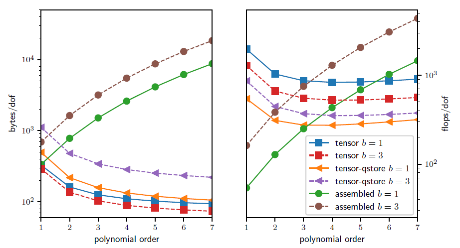
In the right panel, we show the cost in terms of FLOPS/DOF. This metric for computational efficiency made sense historically, when the performance was mostly limited by processors’ clockspeed. A more relevant performance plot for current state-of-the-art high-performance machines (for which the bottleneck of performance is mostly in the memory bandwith) is shown in the left panel, where the memory bandwith is measured in terms of bytes/DOF.
We can see that high-order methods, implemented properly with only partial assembly, require optimal amount of memory transfers (with respect to the polynomial order) and near-optimal FLOPs for operator evaluation.
Thus, high-order methods in matrix-free representation not only possess favorable properties, such as higher accuracy and faster convergence to solution, but also manifest an efficiency gain compared to their corresponding assembled representations.