16) Finite Volume

Last time

• Variational Multiscale Methods

• Streamline Upwind Petrov-Galerkin (SUPG)

• General workflow for time dependent problems

• SUPG solver in Julia

Today

1. Unstructured meshes

2. Finite volume methods for hyperbolic conservation laws
   2.1 Derivation in 1D
   2.2 Non-linearities and shock formation
   2.3 Examples of hyperbolic conservation laws

3. Riemann solvers for scalar equations

4. Shocks and the Rankine-Hugoniot condition

5. Entropy solutions

using LinearAlgebra
using Plots
default(linewidth=3)
using LaTeXStrings

# utility functions for Runge-Kutta ODE time-steppers
struct RKTable
    A::Matrix
    b::Vector
    c::Vector
    function RKTable(A, b)
        s = length(b)
        A = reshape(A, s, s)
        c = vec(sum(A, dims=2))
        new(A, b, c)
    end
end

rk4 = RKTable([0 0 0 0; .5 0 0 0; 0 .5 0 0; 0 0 1 0], [1, 2, 2, 1] / 6)

# explicit RK solver
function ode_rk_explicit(f, u0; tfinal=1., h=0.1, table=rk4)
    u = copy(u0)
    t = 0.
    n, s = length(u), length(table.c)
    fY = zeros(n, s)
    thist = [t]
    uhist = [u0]
    while t < tfinal
        tnext = min(t+h, tfinal)
        h = tnext - t
        for i in 1:s
            ti = t + h * table.c[i]
            Yi = u + h * sum(fY[:,1:i-1] * table.A[i,1:i-1], dims=2)
            fY[:,i] = f(ti, Yi)
        end
        u += h * fY * table.b
        t = tnext
        push!(thist, t)
        push!(uhist, u)
    end
    thist, hcat(uhist...)
end

ode_rk_explicit (generic function with 1 method)

Tip

Some useful resources for FV are:

• Ketcheson, LeVeque, and del Razo, Riemann Problems and Jupyter Solutions - Theory and Approximate Solvers for Hyperbolic PDEs

  • free, Jupyter notebooks python codes

• LeVeque, Finite Volume Methods for Hyperbolic Equations

• Toro, Riemann Solvers and Numerical Methods for Fluid Dynamics

• Conservation Laws package (Clawpack)

1. Unstructured meshes

Some notes on unstructured meshing workflows:

• Many interesting physical or engineering problems are defined on complex geometries. These are hard to model with a regular, structured mesh

• CAD models: spline-based (NURBS) geometry

  • Label materials, boundary surfaces

  • Proprietary formats or lossy open formats

• Geometry clean-up

  • Remove difficult elements/edges/vertices

• Mesh generation

  • Tetrahedral meshing mostly automatic

  • Hexahedral meshes often more efficient (but can make incompressible materials or thin structure suffer from “locking” in elasticity problems)

    • Manually decompose geometry

    • Various algorithms with poor quality elements

  • Usually single node with lots of memory

• Simulation

  • Read, partition, solve, write output

• Load in visualization software (e.g., Paraview, VisIt)

  • Visualization outputs usually contain derived quantities

    • Stress, velocity, pressure, temperature, vorticity

  • Frequent checkpoints are commonly a bottleneck

2. Finite Volume methods for hyperbolic conservation laws

Hyperbolic conservation laws have the form

\[ \frac{\partial \mathbf q}{\partial t} + \nabla\cdot F(\mathbf q) = 0 \]

where the (possibly nonlinear) function \(F(\mathbf q)\) is called the flux.

\(\mathbf q\) represents the local density of some quantity. If \(\mathbf q\) has \(m\) components, \(F(\mathbf q)\) is an \(m\times d\) matrix in \(d\) dimensions.

Similar to what we have seen with the Finite Element Method (FEM), we can express finite volume methods by choosing test functions \(\mathbf v(x)\) that are now piecewise constant (hence, you can think of the Finite Volume method to be a special case of the FEM) on each element \(e\) and integrating by parts (i.e., apply divergence theorem in higher dimensions).

We start by multiplying by the test function and integrating over the domain:

\[ \begin{split} \int_\Omega \left( \mathbf v \frac{\partial \mathbf q}{\partial t} + \mathbf v \nabla\cdot F(\mathbf q) \right) dx = 0\, , \text{ for all } \mathbf v \end{split} \]

We then apply the divergence theorem on the spatial term:

\[ \int_\Omega \mathbf v \nabla\cdot F(\mathbf q) dx = - \int_\Omega \underbrace{ \cancel{ \nabla \mathbf v \cdot F(\mathbf q)}}_{\mathbf v \textrm{ is piecewise const.}} dx + \int_{\partial \Omega} \mathbf v F(\mathbf q) \cdot \hat n ~ ds \, . \]

Because we use piecewise constant test functions \( \mathbf v \) (note the bold type here - if \(\mathbf q\) has \(m\) components, also \(\mathbf v\) has \(m\) components), this is like an indicator function of the computational cell or element \(e\). Hence, for any quantity \(f\), we have

\[ \int_\Omega \mathbf v f = \int_e f \]

and differentiation in time commutes with spatial integration

\[ \begin{split} \frac{\partial}{\partial t} \left( \int_e \mathbf q \right) + \int_{\partial e} F(\mathbf q) \cdot \hat n = 0\, , \text{ for all } e \, , \end{split} \]

where for the spatial term integral we have applied the divergence theorem.

What this tells us:

The rate of change of a given quantity inside a computational cell/volume is balanced by the net flux of that quantity through the boundary of that computational cell/volume.

In general, for Finite Volume methods in any dimension, we choose as our unknowns the average values \(\bar{\mathbf q}\) on each element, leading to the semi-discrete equation

\[ \lvert e \rvert \frac{\partial \bar{\mathbf q}}{\partial t} + \int_{\partial e} F(\mathbf q) \cdot \hat n = 0 \text{ for all } e \]

where \(\lvert e \rvert\) is the volume of element \(e\).

The most basic methods will compute the interface flux in the second term using the cell average \(\bar{\mathbf q}\), though higher order methods will perform a reconstruction using neighbors. Since \(\bar{\mathbf q}\) is discontinuous at element interfaces, we will need to define a numerical flux using the (possibly reconstructed) value on each side.

Let’s see here a more detailed derivation in 1D.

2.1 Derivation in 1D

Start with the 1D conservation law:

(24)\[ u_t + \frac{\partial}{\partial x} f(u) = 0\, , \qquad u(x,0) = u_0(x) \]

For the integral over a computational cell \([x_{i-1/2}, x_{i+1/2}] \equiv [x_L , x_R]\) we have:

\[ \int_{x_{i-1/2}}^{x_{i+1/2}} u_t(x,t)\,dx + \int_{x_{i-1/2}}^{x_{i+1/2}} \frac{\partial}{\partial x} f(u(x,t))\,dx = 0 \]

For the time derivative we have:

\[ \int_{x_{i-1/2}}^{x_{i+1/2}} u_t(x,t)\,dx = \frac{d}{dt} \int_{x_{i-1/2}}^{x_{i+1/2}} u(x,t)\,dx \]

For the flux term (by the Fundamental Theorem of Calculus) we know that:

\[ \int_{x_{i-1/2}}^{x_{i+1/2}} \frac{\partial}{\partial x} f(u(x,t))\,dx = f\big(u(x_{i+1/2}, t)\big) - f\big(u(x_{i-1/2}, t)\big) \]

We then define the cell average:

\[ \bar u_i(t) = \frac{1}{\Delta x} \int_{x_{i-1/2}}^{x_{i+1/2}} u(x,t)\,dx \]

so that:

\[ \int_{x_{i-1/2}}^{x_{i+1/2}} u(x,t)\,dx = \Delta x \,\bar u_i(t) \]

We then substitute this into the integrated equation:

\[ \frac{d}{dt} \big( \Delta x \,\bar u_i \big) + \Big[ f(u_{i+1/2}) - f(u_{i-1/2}) \Big] = 0 \, . \]

Here we should pause for a second. Since we defined the unknown \(u\) averaged over a computational cell, \(\bar u\), do we actually know the values of \(u_{i\pm1/2}\) needed for the flux on the right-hand side?

Observations:

• our unknowns are now cell averages \(\bar u_i\)

• but the flux depends on point values at interfaces

• the way we reconstruct the flux will be the key in the Finite Volume method (via Riemann solvers)

• we will in fact, define a numerical flux as a replacement for the actual flux

Now, since \(\Delta x\) is constant:

\[ \Delta x \,\frac{d \bar u_i}{dt} + f(u_{i+1/2}) - f(u_{i-1/2}) = 0 \]

we can divide by \(\Delta x\):

\[ \frac{d \bar u_i}{dt} = -\frac{1}{\Delta x} \Big( f(u_{i+1/2}) - f(u_{i-1/2}) \Big) \]

We replace the exact flux with a numerical flux, \( \hat f\):

\[ f(u_{i+1/2}) \;\longrightarrow\; \hat f(u_i, u_{i+1}) \]

This gives:

\[ \frac{d \bar u_i}{dt} = -\frac{1}{\Delta x} \Big( \hat f(u_i, u_{i+1}) - \hat f(u_{i-1}, u_i) \Big) \]

The semi-discrete finite volume scheme is:

\[ \frac{d \bar u_i}{dt} = -\frac{1}{\Delta x} \Big( \hat f(u_i, u_{i+1}) - \hat f(u_{i-1}, u_i) \Big) \]

This represents a conservation law at the discrete level:

• \(\hat f(u_{i-1}, u_i)\) = flux entering cell \(i\) from the left

• \(\hat f(u_i, u_{i+1})\) = flux leaving cell \(i\) on the right

So the update is:

\[ \text{rate of change of the averaged quantity} = \text{inflow} - \text{outflow} \]

2.2 Non-linearities and shock formation

We have seen that starting from the 1D initial–value problem for scalar non–linear conservation laws

(25)\[ u_t + \frac{\partial}{\partial x} f(u) = 0\, , \qquad u(x,0) = u_0(x) \]

a corresponding integral form of the conservation law is

(26)\[ \frac{d}{dt} \int_{x_L}^{x_R} u(x,t) dx = f(u(x_L, t)) - f(u(x_R, t)) \, . \]

The flux function \(f\) is assumed to be a function of \(u\) only, which under certain circumstances is an inadequate representation of the physical problem being modelled.

This conservation law can be rewritten more generally as

(27)\[ u_t + \lambda(u) u_x = 0 \, , \qquad u(x,0) = u_0(x) \, . \]

where

(28)\[ \lambda(u) = \frac{df }{du} = f'(u) \]

is the characteristic speed.

• Note: If we had a system of hyperbolic PDEs, then this corresponds to the eigen- values of the Jacobian matrix.

• The behaviour of the flux function \(f(u)\) has profound consequences on the behaviour of the solution \(u(x, t)\) of the conservation law itself.

A crucial property is monotonicity of the characteristic speed \(\lambda(u)\).

There are essentially three possibilities:

• \(\lambda (u)\) is a monotone increasing function of \(u\)

\[ \frac{d \lambda(u)}{du} = \lambda ' (u) = f'' (u) > 0\, \qquad \textrm{ convex flux} \]

• \(\lambda (u)\) is a monotone decreasing function of \(u\)

\[ \frac{d \lambda(u)}{du} = \lambda ' (u) = f'' (u) < 0\, \qquad \textrm{ concave flux} \]

• \(\lambda (u)\) has extrema, for some \(u\)

\[ \frac{d \lambda(u)}{du} = \lambda ' (u) = f'' (u) = 0\, \qquad \textrm{ non-convex, non-concave flux} \]

Construction of solutions on characteristics

Consider characteristic curves \(x = x(t)\) satisfying the IVP

(29)\[ \frac{dx}{dt} = \lambda(u) \, , x(0) = x_0 \, . \]

Then, by regarding both \(u\) and \(x\) to be functions of \(t\) we find the total derivative of \(u\) along the curve \(x(t)\), namely

\[ \frac{d u}{dt} = u_t + \lambda (u) u_x = 0 \, . \]

That is, \(u\) is constant along the characteristic curve satisfying the IVP (29).

More generally, characteristic curves for a PDE are curves along which the equation simplifies in some particular manner - in this case they are lines along which the solution is constant.

Therefore, in this case, the slope \(\lambda (u)\) is constant along the characteristic. Hence, in this case, the characteristic curves are straight lines.

The value of \(u\) along each curve is the value of \(u\) at the initial point \(x(0) = x_0\) and we write

(30)\[ u(x,t) = u_0 (x_0) \, . \]

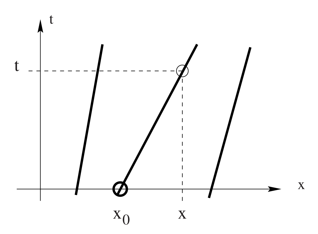
The figure above shows a typical characteristic curve emanating from the initial point \(x_0\) on the \(x\)–axis. The slope \(\lambda (u)\) of the characteristic may then be evaluated at \(x_0\) so that the solution characteristics curves of IVP (29) are

(31)\[ x = x_0 + \lambda (u_0(x_0)) t \, . \]

The last two equations, (30) and (31), may be regarded as the analytical (implicit) solution of the IVP. This is an implicit solution, in fact, it is more apparent if we substitute \(x_0\) from the last equation, in the solution for \(u\):

\[ u(x,t) = u_0 (x - \lambda (u_0 (x_0))t) \,. \]

From (30) we can obtain the \(t\) and \(x\) derivatives

(32)\[ u_t = u_0' (x_0) \frac{\partial x_0}{\partial t} \, , \qquad u_x = u_0' (x_0) \frac{\partial x_0}{\partial x} \]

and from these, we can verify that the relations (30) and (31) actually define the solution (as \(u_t\) and \(u_x\) satisfy the PDE (27)).

2.3 Examples of hyperbolic conservation laws

Advection

\[ \frac{\partial u}{\partial t} + \nabla\cdot (\underbrace{a u}_{F(u)}) = 0 \]

where \(a\) is the propagation speed.

In the absence of boundary conditions, this has the solution

\[ u(t,x) = u(0, x-at) \]

in terms of the initial condition.

We have seen already that lines of constant \(u\), \(x-at\) are called characteristics.

• The wave speed is, in this case, \(F'(u) = a\), a constant. Hence the solution consists of the initial data \(u_0 (x)\) translated with speed \(a\) without distortion.

• For nonlinear cases instead, the characteristic speed \(\lambda(u)\) is a function of the solution \(u\) itself. Distortions are therefore produced; this is a distinguishing feature of nonlinear problems.

Burger’s Equation

\[ \frac{\partial u}{\partial t} + \nabla\cdot \underbrace{\left(\frac{u^2}{2}\right)}_{F(u)} = 0 \]

is a model for nonlinear convection.

• The wave speed is \(F'(u) = u\) (thus, it increases as \(u\) increases).

Traffic model

A general, simple traffic flow model is

\[ \frac{\partial u}{\partial t} + \nabla\cdot \big(\underbrace{u (1-u)}_{F(u)} \big) = 0 \]

where \(u \in [0,1]\) represents local traffic density of cars on a straight, single-lane road aligned with the \(x\)-axis and \((1-u)\) is their speed.

• The characteristic speed is \(F'(u) = 1 - 2u\), representing the speed at which kinematic waves travel.

• This is a non-convex or concave flux function.

In 1D, if we expand

\[ \frac{\partial u}{\partial t} + \frac{\partial}{\partial x} \big(u -u^2) = 0 \, \]

and apply the chain rule

\[ u_t + (1- 2u) u_x = 0 \, \]

we find what is called a quasilinear form. It’s quasilinear because is linear in the highest-order spatial derivative of the unknown (\(u_x\) in this case), but is not linear for the dependent variable \(u\).

3. Riemann solvers for scalar equations

First crack at a numerical flux

Problem: We represent the solution in terms of cell averages \(\bar u\), but need to compute

\[ \int_{\partial e} F(u) \cdot \hat n ds \]

on the boundary of each cell (i.e., in higher-dimensions, on each edge/face).

For interior faces, the flux \(F(u)\) must be the same when viewed from either side.

As a first idea for an accurate numerical method, we could consider \(u\) at the element interface to be the average of the values from the left and right side of each face,

\[ u_{\text{face}} = \frac{\bar u_L + \bar u_R}{2} . \]

Let’s try that.

function testfunc(x)
    max(1 - 4*abs.(x+2/3),
        abs.(x) .< .2,
        (2*abs.(x-2/3) .< .5) * cospi(2*(x-2/3)).^2
    )
end
plot(testfunc, xlims=(-1, 1), legend=:none)

An implementation in Julia

flux_advection(u) = u
flux_burgers(u) = u^2/2
flux_traffic(u) = u * (1 - u)

function fv_solve0(flux, u_init, n, tfinal=1)
    h = 2 / n # 1D domain [-1,1]
    x = LinRange(-1+h/2, 1-h/2, n) # cell midpoints (centroids)
    idxL = 1 .+ (n-1:2*n-2) .% n # left interface indices
    idxR = 1 .+ (n+1:2*n) .% n # right interface indices
    function rhs(t, u)
        uL = .5 * (u + u[idxL])
        uR = .5 * (u + u[idxR])
        (flux.(uL) - flux.(uR)) / h
    end
    thist, uhist = ode_rk_explicit(rhs, u_init.(x), h=h, tfinal=tfinal)
    x, thist, uhist
end

fv_solve0 (generic function with 2 methods)

x, thist, uhist = fv_solve0(flux_traffic, testfunc, 100, .2)
plot(x, uhist[:,1:5:end], label=[L"t_0" L"t_5" L"t_{10}"], xlabel = "x", ylabel = "u") # checkpoint the solution at every 5th time step

Evidenitly our method has serious problems for discontinuous, non-smooth solutions and nonlinear problems.

4. Shocks and the Rankine-Hugoniot condition

Shocks, rarefactions, and Riemann problems

Burger’s equation evolves a discontinuity in finite time from a smooth initial condition.

It turns out that all nonlinear hyperbolic equations have this property.

For Burgers, the peak travels to the right, steepening, and eventually overtaking the troughs (like in ocean waves).

• This is called a shock and corresponds to characteristics converging when the gradient of the solution is negative. In this case we have a breakdown of the solution.

• When the gradient of the solution is positive, the characteristics diverge to produce a rarefaction, which is, a reduction of density (a common rarefaction wave is the area of low relative pressure following a shock wave).

The relationship to positive and negative gradients is reversed for a non-convex flux like in the Traffic model.

We need a solution method that can correctly compute fluxes in case of a discontinuous solution.

Finite volume methods represent this in terms of a Riemann problem: two constant states separated by a discontinuity

\[\begin{split} u(0, x) = \begin{cases} u_L , & \text{if} & x < 0 \\ u_R , & \text{if} & x > 0 \end{cases} \end{split}\]

where \(u_L\) and \(u_R\) are given.

The solution of a Riemann problem is the solution \(u(t, x)\) at positive times.

More generally, the Riemann problem consists of the hyperbolic equation together with special initial data that is piecewise constant with a single jump discontinuity. We expect this discontinuity to propagate along the characteristic curves.

In our finite volume schemes, it will be sufficient to compute the flux at \(x=0\) at an infinitesimal positive time

\[ \tilde F(u_L, u_R) = \lim_{t\to 0} F\big(u(t, 0) \big) . \]

We call \(\tilde F\) the numerical flux and require that it must be consistent when there is no discontinuity,

\[ \tilde F(u, u) = F(u) .\]

A solver based on Riemann problems

riemann_advection(uL, uR) = 1*uL # velocity is +1

function fv_solve1(riemann, u_init, n, tfinal=1)
    h = 2 / n # 1D domain [-1,1]
    x = LinRange(-1+h/2, 1-h/2, n) # cell midpoints (centroids)
    idxL = 1 .+ (n-1:2*n-2) .% n # left interface indices
    idxR = 1 .+ (n+1:2*n) .% n # right interface indices
    function rhs(t, u)
        fluxL = riemann(u[idxL], u)
        fluxR = riemann(u, u[idxR])
        (fluxL - fluxR) / h
    end
    thist, uhist = ode_rk_explicit(rhs, u_init.(x), h=h, tfinal=tfinal)
    x, thist, uhist
end

fv_solve1 (generic function with 2 methods)

x, thist, uhist = fv_solve1(riemann_advection, testfunc, 400, .1)
plot(x, uhist[:,1:5:end], legend=:none)

Observations

• Good: no oscillations/noisy artifacts: solutians are bounded between 0 and 1, just like the exact solution.

• Bad: Lots of numerical diffusion (amplitudes are damped).

Rankine-Hugoniot condition

We go back to the conservation law in integral form (26). Enforcing the conservation on an arbitrary control volume/cell \([x_L, x_R]\) leads to

\[ f(u(x_L,t)) - f(u(x_R,t)) = \frac{d}{dt} \int_{x_L}^{s(t)} u(x,t) dx + \frac{d}{dt} \int_{x(s)}^{x_R} u(x,t) dx \, . \]

Using Leibniz integral rule, we can write this as

\[ f(u(x_L,t)) - f(u(x_R,t)) = [u(s_L,t) -u(s_R,t)]S + \int_{x_L}^{s(t)} u_t(x,t) dx + \int_{x(s)}^{x_R} u_t(x,t) dx \, , \]

where \(u(s_L , t)\) is the limit of \(u(s(t), t)\) as \(x\) tends to \(s(t)\) from the left, \(u(s_R , t)\) is the limit of \(u(s(t), t)\) as \(x\) tends to \(s(t)\) from the right and \(S = ds/dt\) is the speed of the shock/discontinuity.

Since \(u_t(x,t)\) is bounded the integrals vanish identically as \(s(t)\) is approached from left and right and we obtain

\[ f(u(x_L,t)) - f(u(x_R,t)) = [u(s_L,t) -u(s_R,t)]S \, . \]

This tells us that:

If we move into the reference frame of the shock, the flux on the left must be equal to the flux on the right.

More generally, in any dimension (where we have denoted the flux by \(F\)), we rewrite the equation that the shock speed \(S\) satisfies as

\[ S (\underbrace{u_R - u_L}_{\Delta u}) = (\underbrace{F(u_R) - F(u_L)}_{\Delta F}) \cdot \hat n \]

where \(\hat n\) is any direction (e.g., the normal to a face in a multi-dimensional finite volume method).

Or:

\[ S = \frac{\Delta F}{\Delta u} \, . \]

This condition holds also for hyperbolic system.

For Burger’s equation

\[ \frac{\partial u}{\partial t} + \nabla\cdot (u^2/2) = 0, \]

\[\begin{split} u(x,0) = u_0(x) = \begin{cases} u_L , & x < 0 \\ u_R , & x > 0 \end{cases} \end{split}\]

Let’s analyze different scenarios.

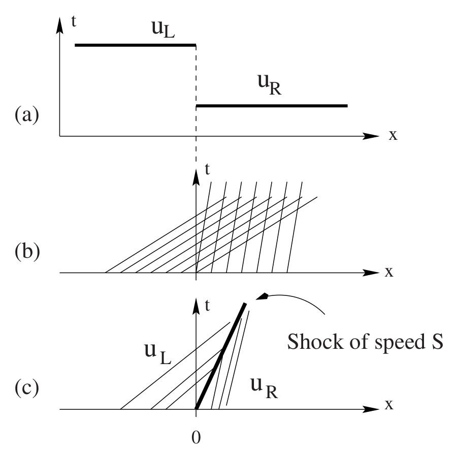
• If \(u_L > u_R\), i.e., \(\Delta u < 0\). As the flux is convex, \(\lambda ' (u) = F'' (u) > 0\) characteristic speeds on the left are greater than those on the right. That is, \(\lambda_L \equiv \lambda(u_L) > \lambda_R \equiv \lambda (u_R) \).

The disconinous solution of the IVP in this case is

\[\begin{split} u(x,t) = \begin{cases} u_L , & \textrm{ if } x - St < 0 \\ u_R , & \textrm{ if } x - St > 0 \end{cases} \end{split}\]

For this case, the shock propagates at speed

\[ S = \frac{\Delta F}{\Delta u} = \frac{ \frac{u_R^2}{2} - \frac{u_L^2}{2} }{ u_R - u_L} = \frac{ u_R^2 - u_L^2}{2 (u_R - u_L)} = \frac{\cancel{(u_R - u_L)} (u_R + u_L)}{2 \cancel{(u_R - u_L)}} = \frac{(u_R + u_L)}{2} \]

In this case, since \(u_L > u_R\), then \(u_L^2 / 2 > u_R^2 /2 \), hence, \(F(u_L) > F(u_R)\), or \(\Delta F < 0\), and therefore \(S>0\), which tells us that the shock moves to the right, and the characteristic lines interesct immediately (compressive region).

The solution in this case satisfies the following condition

(33)\[ \lambda (u_L) \equiv F'(u_L) > S > \lambda (u_R) \equiv F'(u_R) \]

which is called the entropy condition.

So if the solution is a shock, the numerical flux is the maximum of \(f(u_L)\) and \(f(u_R)\).

We still don’t know what to do in case of a rarefaction so will just average and see what happens.

Burgers Riemann problem (shock)

function riemann_burgers_shock(uL, uR)
    flux = zero(uL)
    for i in 1:length(flux)
        flux[i] = if uL[i] > uR[i] # shock
            max(flux_burgers(uL[i]), flux_burgers(uR[i]))
        else
            flux_burgers(.5*(uL[i] + uR[i])) # in this case, we take the average
        end
    end
    flux
end

riemann_burgers_shock (generic function with 1 method)

x, thist, uhist = fv_solve1(
    riemann_burgers_shock, cospi, 100, 1)
plot(x, uhist[:,1:10:end], legend=:none)

Rarefactions

This solution was better, but we still have odd ripples in the rarefaction.

• If \(u_L < u_R\)

This data is the extreme case of expansive data, for convex \(f(u)\). A possible mathematical solution to the PDE (not really a physical solution) has the same form as for the compressive data case. Its charactestistics would look like in the figure below.

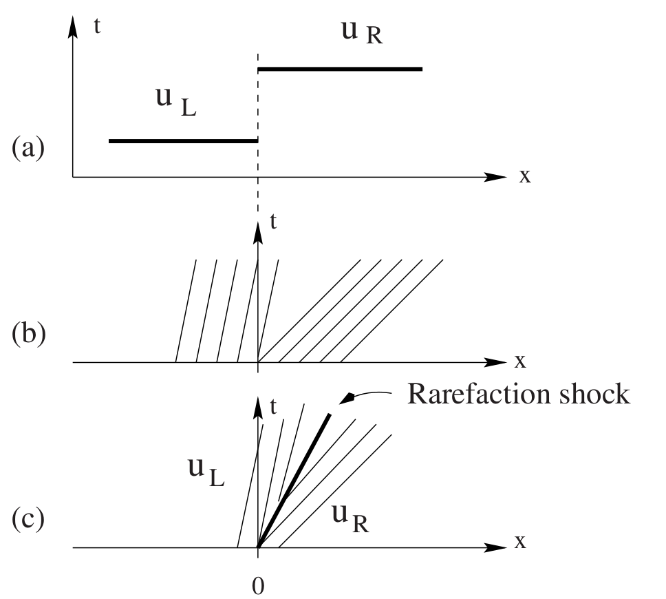
However, this solution is physically incorrect. In this case, the discontinuity does not arise because of compression, i.e., \(\lambda_L < \lambda_R\); the characteristics diverge from the discontinuity. This solution is called a rarefaction shock, or entropy-violating shock, and does not satisfy the entropy condition

\[ F'(u_L) > S > F'(u_R) \]

or, more simply

\[ F'(u_L) > F'(u_R) \, .\]

Shocks are compressive phenomena and physical solutions to the opposite, expansive scenario

\[ F'(u_L) < F'(u_R) \]

are instead rarefactions.

• Shocks appear in regions where characteristics converge.

• Rarefactions appear in regions where characteristics are spreading out.

Physical rarefaction waves

Consider again the IVP with general convex flux function \(f(u)\)

\[ u_t + f(u)_x = 0\, , \]

(34)\[\begin{split} u(x,0) = u_0(x) = \begin{cases} u_L , \, & x < 0 \\ u_R , \, & x > 0 \end{cases} \end{split}\]

and expansive initial data, \(u_L < u_R\). As discussed, we have found a solution that is not physical. An entropy-violating for this problem would be:

(35)\[\begin{split} u(x,t) = \begin{cases} u_L & \text{ if } & x - St < 0\\ u_R & \text{ if } & x - St > 0 \end{cases} \end{split}\]

with

\[ S = \frac{\Delta f}{\Delta u} \, . \]

Amongst the various other reasons for rejecting this solution as a physical solution, instability stands out as a prominent argument. By instability it is meant that “small perturbations of the initial data lead to large changes in the solution”.

If we modify the initial data of the IVP to have a transition between the \(u_L\) and \(u_R\) values via a “ramp” function, like in the figure below:

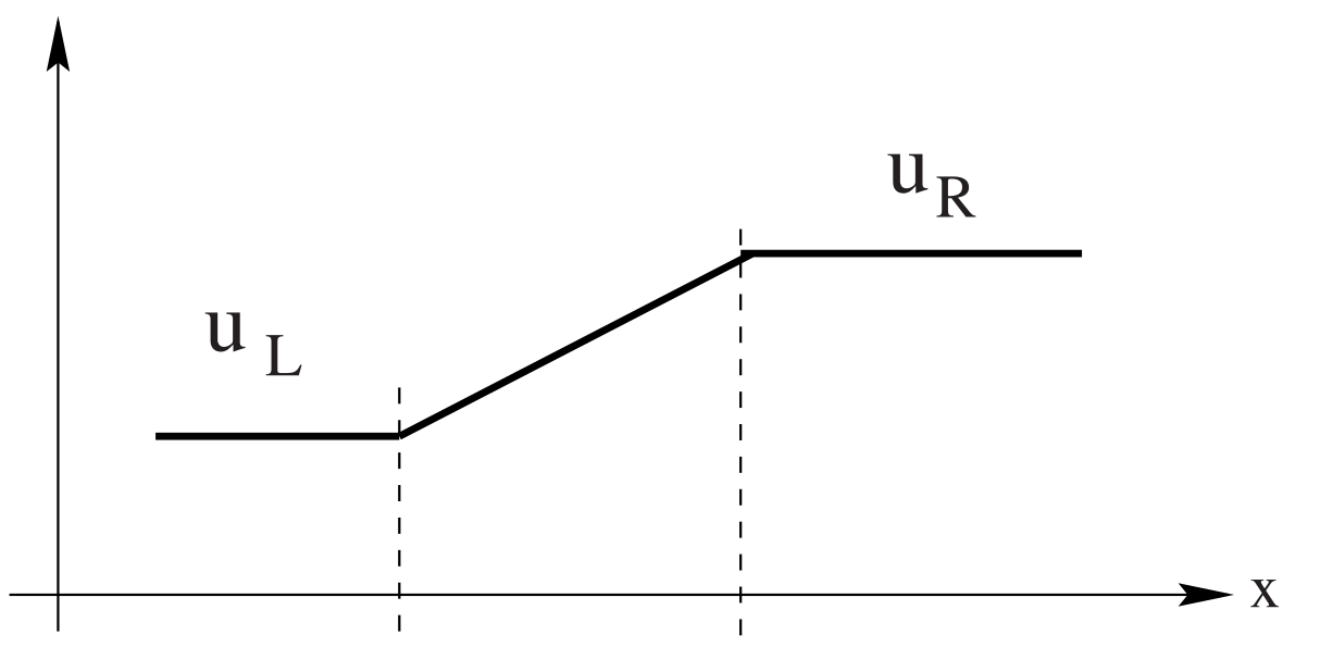
Now we have replaced the discontinuous change from \(u_L\) to \(u_R\) by a linear variation of \(u_0 (x)\) between two fixed points, \(x_L < 0\) and \(x_R > 0\). We use the \(2\)-point formula for a line between two points \((x_L,u_L)\), and \((x_R,u_R)\), and the new initial data is:

\[\begin{split} u_0(x) = \begin{cases} u_L , & \text{if} & x \leq x_L \\ u_L + \frac{u_R - u_L}{x_R - x_L}(x - x_L) & \text{if} & x_L < x < x_R \\ u_R & \text{if} & x \geq x_R \end{cases} \end{split}\]

The solution \(u(x, t)\) to this problem is found by following characteristics, as discussed previously, and consists of two constant states, \(u_L\) and \(u_R\) , separated by a region of smooth transition between the data values \(u_L\) and \(u_R\). This is called a rarefaction wave.

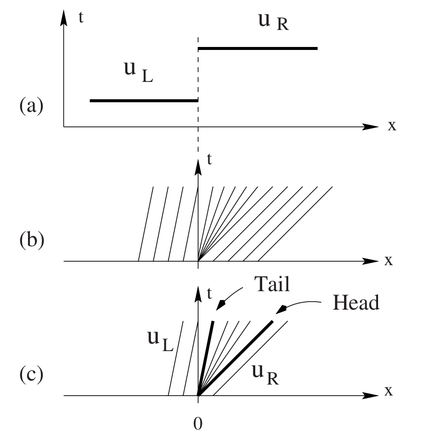
The right edge of the wave is given by the characteristic emanating from \(x_R\)

\[ x = x_R + \lambda(u_R) t \]

and is called the “head” of the rarefaction wave. It carries the value \(u_0(x_R) = u_R\).

The left edge of the wave is given by the characteristic emanating from \(x_L\)

\[ x = x_L + \lambda(u_L) t \]

and is called the “tail” of the rarefaction wave. It carries the value \(u_0(x_L) = u_L\).

As we assume convexity, \(\lambda ' (u) = f '' (u) > 0\), larger values of \(u_0 (x)\) propagate faster than lower values and thus the wave spreads and flattens as time evolves. The spreading of waves is a typical nonlinear phenomenon not seen in the study of linear hyperbolic systems with constant coefficients.

The entire solution is

\[\begin{split} \begin{align*} u(x,t) &= u_L & \text{ if } & \quad \frac{x - x_L}{t} \leq \lambda_L \, \\ \lambda(u) &= \frac{x - x_L}{t} & \text{ if } & \quad \lambda_L < \frac{x - x_L}{t} < \lambda_R \, \\ u(x,t) &= u_R & \text{ if } & \quad \frac{x-x_R}{t} \geq \lambda_R \, . \end{align*} \end{split}\]

No matter how small the size \(\Delta x = x_R - x_L\) of the interval over which the discontinuous data in IVP (34) has been spread over, the structure of the above rarefaction solution remains unaltered and is entirely different from the rarefaction shock solution (35), for which small changes to the data lead to large changes in the solution.

From the above construction the rarefaction solution is instead stable and as \(x_L\) and \(x_R\) approach zero from below and above respectively, the discontinuous data at \(x = 0\) in IVP (34) is reproduced.

Therefore, the limiting case is to be interpreted as follows: \(u_0 (x)\) takes on all the values between \(u_L\) and \(u_R\) at \(x = 0\) and consequently \(\lambda(u_0 (x))\) takes on all the values between \(\lambda_L\) and \(\lambda_R\) at \(x = 0\). As higher values propagate faster than lower values the initial data disintegrates immediately giving rise to a rarefaction solution. This limiting rarefaction in which all characteristics of the wave emanate from a single point is called a centred rarefaction wave (like the one in the figure above).

In this case we need to color into the rarefaction in a physical way. We can justify this by considering the hyperbolic problem to be the singular limit of a problem with diffusion/viscosity, leading to “viscosity solutions”.

Looking into the rarefaction fan

# satisfying now both the Rankine-Hugoniot and entropy conditions
function riemann_burgers(uL, uR)
    flux = zero(uL)
    for i in 1:length(flux)
        fL = flux_burgers(uL[i])
        fR = flux_burgers(uR[i])
        flux[i] = if uL[i] > uR[i] # shock
            max(fL, fR)
        elseif uL[i] > 0 # rarefaction all to the right
            fL
        elseif uR[i] < 0 # rarefaction all to the left
            fR
        else
            0
        end
    end
    flux
end

riemann_burgers (generic function with 1 method)

x, thist, uhist = fv_solve1(
    riemann_burgers, cospi, 100, 1)
plot(x, uhist[:,1:10:end], legend=:none)

5. Entropy solutions

Consider a smooth function \(\eta(u)\) that is convex \(\eta''(u) > 0\) and a smooth solution \(u(t,x)\). Then

\[ u_t + F(u)_x = 0 \]

is equivalent to

\[ u_t + F'(u) u_x = 0 \]

(where we have just expanded using the chain rule) and we can multiply this equation by \(\eta'(u)\), obtaining

\[ \eta'(u) u_t + \eta'(u) F'(u) u_x = 0 . \]

If we find a function \(\psi(u)\) such that \(\psi'(u) = \eta'(u) F'(u)\), the equation above is equivalent (for smooth solutions) to

\[ \eta(u)_t + \psi(u)_x = 0 \]

which is a conservation law for the entropy \(\eta(u)\) with entropy flux \(\psi(u)\).

Now consider the parabolic equation

\[ u_t + F(u)_x -\epsilon u_{xx} = 0 \]

for some positive \(\epsilon\).

This equation has a smooth solution for any \(\epsilon > 0\) and \(t > 0\) so we can multiply by \(\eta'(u)\) as above and apply the chain rule to yield

\[ \eta(u)_t + \psi(u)_x - \epsilon \eta'(u) u_{xx} = 0 . \]

Rearranging the last term produces

\[ \eta(u)_t + \psi(u)_x - \epsilon \Big( \eta'(u) u_x \Big)_x = - \epsilon \eta''(u) u_x^2 . \]

If both terms involving \(\epsilon\) were to vanish, we would be left with conservation of entropy.

Entropy solutions: \(\epsilon\to 0\)

We have reached

\[ \eta(u)_t + \psi(u)_x - \epsilon \Big( \eta'(u) u_x \Big)_x = - \epsilon \eta''(u) u_x^2 \]

Because \(\eta(u)\) is convex, \(\eta''(u) > 0\), hence the right-hand side of the equation above is always \( \leq 0\). In fact, any added viscosity causes entropy to decrease, not increase.

Left side

\[ \int_a^b \Big( \eta'(u) u_x \Big)_x dx = \eta'(u) u_x |_{x=a}^b \]

which is bounded independent of the values \(u_x\) may take inside the interval. Consequently, the left hand side reduces to a conservation law in the limit \(\epsilon\to 0\).

Right side

The integral of the right hand side, however, does not vanish in the limit since

\[ \int_a^b u_x^2 \]

is unbounded as \(u_x\) grows near a forming shock.

• again, \(\eta(u)\) being convex implies \(\eta''(u) > 0\).

So entropy must be dissipated across shocks,

\[ \eta(u)_t + \psi(u)_x \le 0, \]

with equality for smooth solutions and strict inequality at shocks.

Mathematical versus physical entropy

Our choice of \(\eta(u)\) being a convex function \(\eta''(u) > 0\) causes entropy to be dissipated across shocks. This is the convention in math literature because convex analysis chose the sign (versus “concave analysis”).

Physical entropy is produced by such processes, so \(-\eta(u)\) would make sense as a physical entropy.

Uniqueness

While any convex function will work to show uniqueness for scalar conservation laws, that is not true of hyperbolic systems, for which the “entropy pair” \((\eta, \psi)\) should satisfy a symmetry property. A “physical entropy” exists for real systems, and may be used for this purpose.

Example: Shallow-water equations

\[\begin{split}\begin{bmatrix} h \\ h\mathbf u \end{bmatrix}_t + \nabla\cdot\begin{bmatrix} h\mathbf u \\ h \mathbf u \otimes \mathbf u + \frac{g}{2} h^2 \mathbf I \end{bmatrix} = 0\end{split}\]

• conserve mass and momentum

• energy is only conserved for smooth solutions

• shocks (crashing waves) produce heat, but energy is not a state variable.

• Energy is the “entropy” of shallow water

  \[ \eta = \underbrace{\frac h 2 \lvert \mathbf u \rvert^2}_{\text{kinetic}} + \underbrace{\frac g 2 h^2}_{\text{potential}}\]

Preview: Riemann problem for the Euler equations

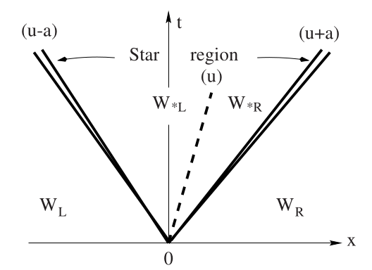
• Two nonlinear (acoustic) waves

  • Either is a shock or rarefaction

• One linearly degenerate (contact) wave

  • Not a shock or rarefaction

  • Pressure is constant across the contact wave

  • Different temperature and density

• Need to determine the wave structure to sample the flux.