3) Introduction to PDEs#
Last time:
Introduction to Community Projects
Today:
Introduction to PDEs
Classification of PDEs
2.1 Generalization
2.2 Examples
1. Introduction to PDEs#
What are PDEs?#
Partial Differential Equations (PDEs) are equations involving a multivariate function, e.g, \(u(x_1, x_2, \ldots, x_n) = u(\mathbf{x})\) and one or more of its (partial) derivatives.
A PDE can be time depedent, i.e, \(u(t, x_1, x_2, \ldots, x_n) = u(t, \mathbf{x})\) or not.
Commonly occurring terms and notation#
Vector Calculus and Differential Geometry#
A scalar-valued function (or scalar field) of several variables (i.e., multivariate) is a function \(u(\mathbf x ): \mathbb{R}^n \to \mathbb{R}\).
A vector-valued function (or vector field) is a function whose range (or codomain) is in multiple dimensions, regardless of the domain dimensions. That is, it could be a function of one (\(\mathbf u(x)\)) or more variables (\(\mathbf u(\mathbf x)\)) such that \(\mathbf u(x): \mathbb{R} \to \mathbb{R}^n\) or \(\mathbf u(\mathbb{\mathbf x}): \mathbb{R}^n \to \mathbb{R}^n\).
For a scalar-valued function \(u(\mathbf x): \mathbb{R}^n \to \mathbb{R}\), the gradient \(\nabla u(\mathbf x)\)
maps vector field to vector field, that is \(\nabla u(\mathbf x): \mathbb{R}^n \to \mathbb{R}^n\)
For a vector-valued function \(\mathbf u(\mathbb{\mathbf x}): \mathbb{R}^n \to \mathbb{R}^n \), Curl \(\mathbf u\) or \(\nabla\times \mathbf u(\mathbf x)\)
maps vector field to vector field, \(\mathbb{R}^n \to \mathbb{R}^n\), that is, \(\nabla\times \mathbf u(\mathbf x): \mathbb{R}^n \to \mathbb{R}^n\)
Divergence of a vector field \(div \mathbf u(\mathbf x) = \nabla\cdot \mathbf u(\mathbf x)\)
maps vector field to scalar field, that is \( \nabla\cdot \mathbf u(\mathbf x):\mathbb{R}^n \to \mathbb{R}\)
Laplacian of a twice-differentiable scalar field \(\Delta u := \nabla \cdot \nabla u \equiv div(\nabla u)=\nabla^2 u\)
maps scalar field to scalar field, that is \(\nabla^2 u: \mathbb{R} \to \mathbb{R}\)
time derivatives: \(\frac{\partial u(t, \mathbf x)}{\partial t}\)
What do PDEs describe?#
A plethora of phenomena. For example:
heat transfer
electrostatics, electromagnetics
solid mechanics
fluid mechanics
quantum mechanics
population dynamics
Classes of methods we’ll cover#
At grid points with rules to approximate derivatives
Finite Difference / collocation
A weak (integral) over elements with rules to reconstruct from element averages and define fluxes
Finite Volume
A weak form over elements with solution and “test functions” in the same space
Finite Element / Galerkin
Examples:#
Viscous Burgers’ Equation#
Viscous Burgers’ equation
It is an example of convection–diffusion equation.
There has been a large amount of work done on the above equation. There is an exact solution to this problem. For the purposes of this course, it is probably better to try to work with this problem without knowing the exact solution since that is the situation in which a working numerical analysit must function.
Inviscid Burgers’ Equation#
Equivalent to the problem above, but without the viscosity term (i.e., for \(\nu = 0\)):
We note that the only difference between the inviscid and the viscous Burger’s equation is that the \(v_{xx}\) term is not included in the inviscid form.
As we shall see later, this difference theoretically changes the whole character of the problem.
We also note that this problem is well-posed with a boundary condition at both endpoints of the domain, \(x=0\) and \(x=1\).
Variable-coefficients Poisson’s equation#
A variable-coefficients (often with discontinuities) Poisson’s problem. This problem can have many important applications ranging from incompressible flows to semiconductor modeling to tissue engineering.
Find \(u\) such that
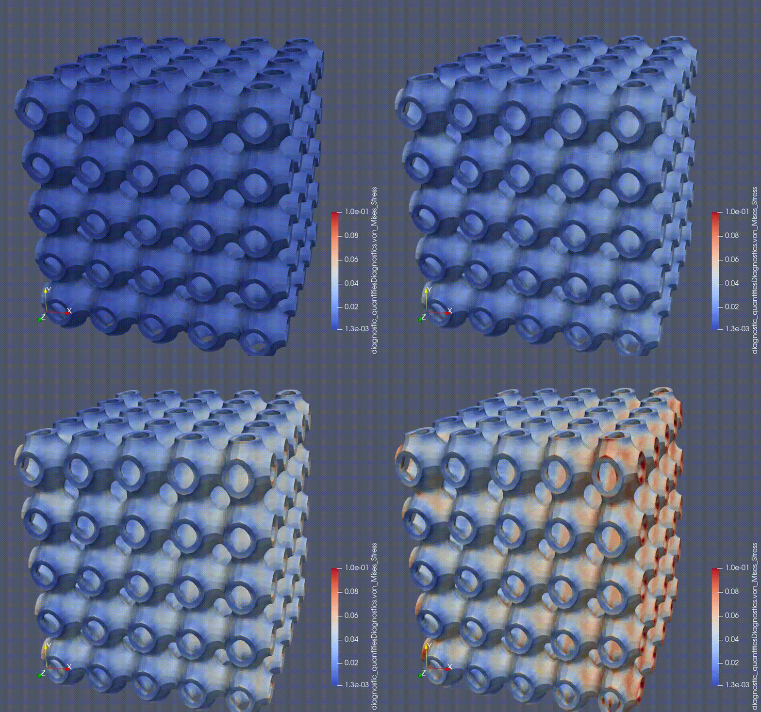
Structural mechanics applications#

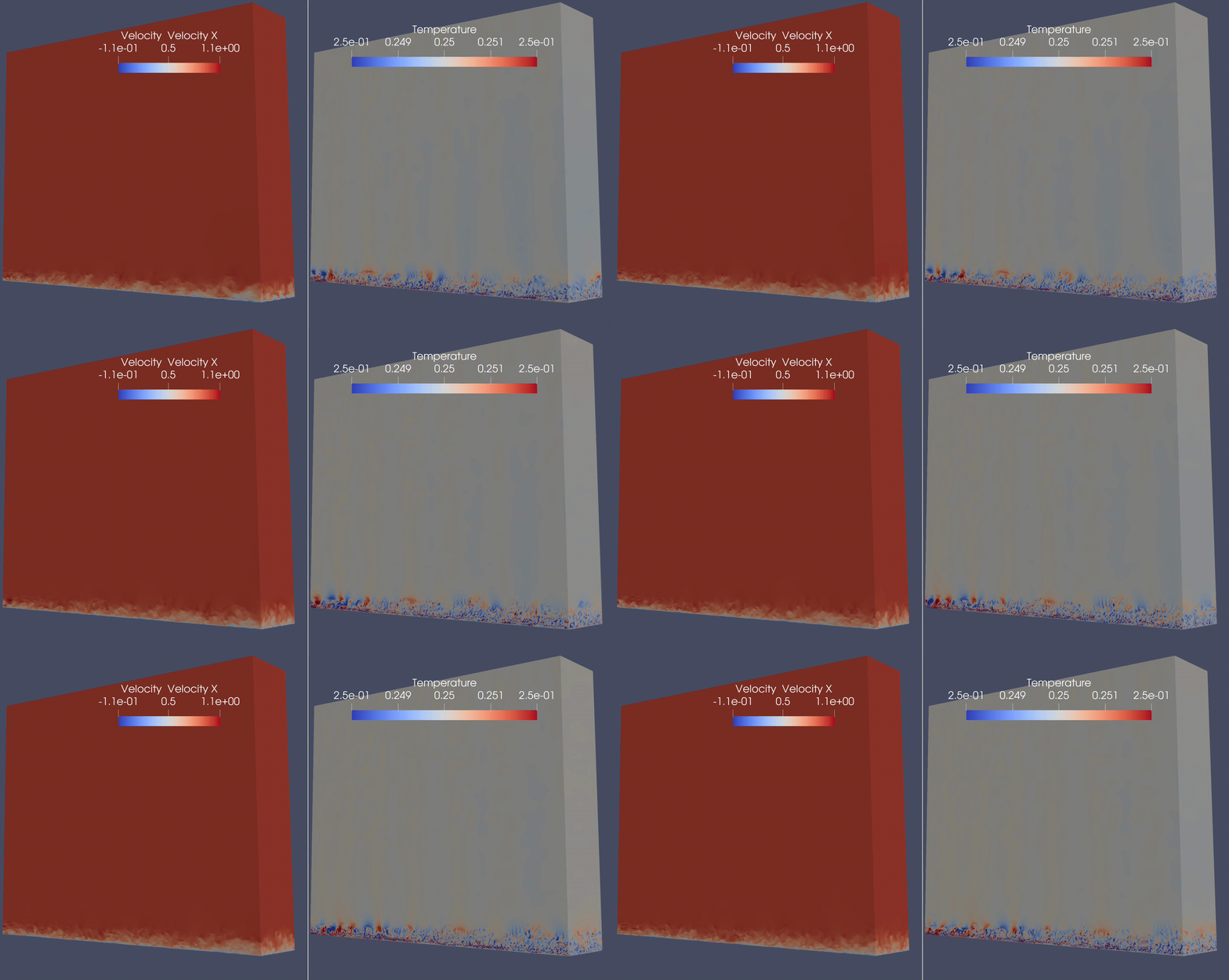
Computational Fluid Dynamics (CFD) applications#

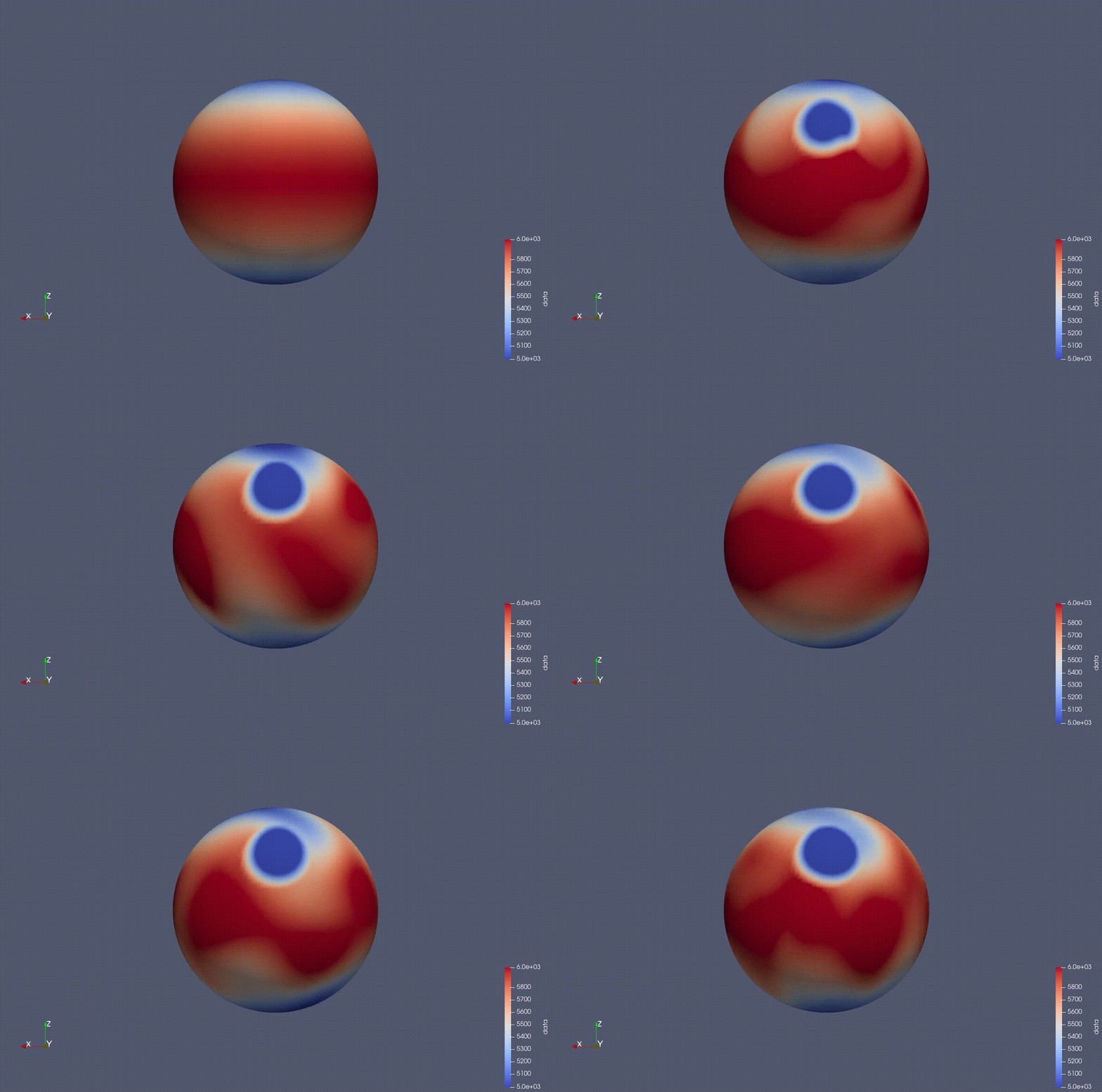
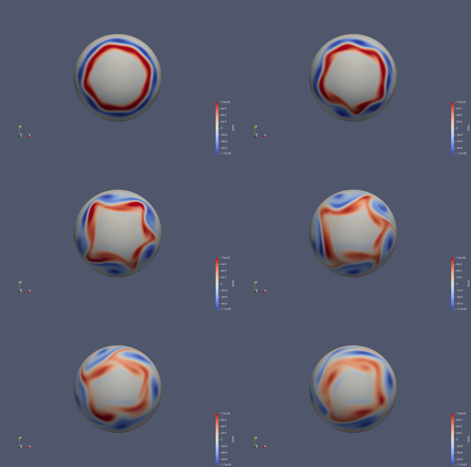
Atmospheric Flow simulations (for numerical weather or climate predictions)#
The shallow water equations (SWE)#
The shallow water equations (in vector-invariant form) on a rotating sphere:
where \(f\) is the Coriolis term and \( \Phi = g (h+h_s) \), and \(h\) is the height function relative to a fixed substrate \(h_s\).


How expensive is it?#
Suppose our domain is \(\Omega = (0, 1)^3\)
We discretize it by dividing each side into segments of length \(h\) (\(n := 1/h\) of them)
We have a total of \(N := n^3\) volume elements
Assume:
Method whose error goes as \(10 h^4\)
Implementation 1 of this method whose runtime scales \(\propto N = n^3\)
Implementation 2 (less efficient) scales \(\propto N^2 = n^6\)
We say \(\mathcal{O}(N)\) and \(\mathcal{O}(N^2)\), respectively
Error vs \(n\) (or \(h\)) is the convergence of a method
Computational cost (e.g. runtime) vs \(n\) is the complexity of the method
In practice, the most important plot is error vs computational cost (work-precision diagram). Why?
Let’s see it for our two methods
using Pkg
Pkg.add("Plots") # let's add the package Plots to our environment

using Plots # once added, you need to import it into your file to e able to use it
default(linewidth=4)

using Pkg; Pkg.add("LaTeXStrings") # let's add the package LaTeXStrings to our environment
using LaTeXStrings # this way we can have nice math in plot legends/titles
Updating registry at `~/.julia/registries/General.toml`
Resolving package versions...
  No Changes to `~/.julia/environments/v1.10/Project.toml`
  No Changes to `~/.julia/environments/v1.10/Manifest.toml`
┌ Warning: Circular dependency detected.
│ Precompilation will be skipped for dependencies in this cycle:
│  ┌ Symbolics → SymbolicsForwardDiffExt
│  └─ Symbolics → SymbolicsPreallocationToolsExt
└ @ Pkg.API.Precompilation ~/julia-1.10.10/share/julia/stdlib/v1.10/Pkg/src/precompilation.jl:583
# An example with a common "good" discretization
error(h) = min(1, 10*h^4)

function cost(h) # a model for algorithmic cost
    n = 1/h # number of points per dimension
    N = n^3 # total number of grid points in 3D
    N # the return value
end

function cost2(h) # another model for algorithmic cost
    N = cost(h)
    N^2 # it is the square of the previous model cost
end
cost2 (generic function with 1 method)
plot([cost, cost2], error, .01, 1, xscale=:log10, yscale=:log10,
  xlabel="Cost", ylabel="Error", label = [L"\mathcal{O}(N)" L"\mathcal{O}(N^2)"])
How to interpret this plot:
To achieve an error of \(10^{-4}\), method 2 needs much more computational resources
This graph lets you read off exactly how expensive the computation will be for a given accuracy (how long you have to wait, your usage)
What goes in? What comes out?#
In:
Equations
Conservation
Variational principles
Materials
Geometry
meshing needed?
Boundary conditions
essential/Dirichlet
natural/Neumann
mixed
Initial conditions
Out:
Discrete solutions
Sampled on a grid
Time series
Quantities of Interest (QoI)
Heat flux
Maximum temperature
Maximum stress
Lift, drag
Eigensolutions
Resonant frequencies/modes
Orbitals
Who works with PDE solvers?#
Numerical analysts
Domain scientists and engineers
Materials scientists
HPC specialists
Optimizers
Statisticians
What skills should they have?#
Breakout groups: pick one role and make a list of essential and nice-to-have skills, plus at least one question. Pick one member to report out.
…
…
2. Classification of PDEs#
A second-order PDE (i.e., a PDE involving second order partial derivatives) in two independent variables \((x,y)\) takes the general form
The coefficients \(a\), \(b\), \(c\), \(d\), \(e\), \(f\), and \(g\) are here (for now) assumed to be functions of the independent variables \((x,y)\) only, so the equation is linear (for the dependent variable, the unknown \(u = u(x,y)\)).
Note
In some textbooks, you can find the convention of the \(xy\) term coefficient being \(2b\) rather than \(b\).
Definitions
A PDE is called linear if it is linear in the unknown and its derivatives.
If the right-hand-side (RHS) term \(g\) (i.e., the known term that does not involve the unknown \(u\)) is equal to zero, the PDEs is said to be homogeneous. Otherwise, if \(g \neq 0\), it is inhomogeneous.
If the coefficients are such that \(a(x,y)\equiv a, b(x,y)\equiv b, \dots\), the PDE is said to be with constant coefficients. Otherwise, with non-constant coefficients.
Let’s consider a homogeneous, constant coefficients second-order PDE in the general form:
This long expression is reminiscent of the formula for the most general conic section. Indeed, we can see that through a change of variables
This change of variable is formally done by a Fourier transform (we’ll see this later in the course). Then we get exactly the conic section equation:
We have converted the constant-coefficient PDE into a polynomial of the same degree, with the terms of the highest degree (a homogeneous polynomial, here a quadratic form) being most significant for the classification.
Now recall from analytic geometry that it is always possible to make a rotation of axes in the \(X–Y\) space after which the cross-term (\(XY\)) coefficient \(b\) is zero.
Suppose that this has been done, we reach the canonical form:
Then recall that (if certain “degenerate cases” are ignored) the curve described by this equation is an
We have three main canonical form classifications:
Just as one classifies conic sections and quadratic forms into hyperbolic, parabolic, and elliptic based on the discriminant \(b^2 − 4ac\), the same can be done for a second-order PDE at a given point. Note that in most textbooks, the general form of a PDE is with the \(xy\) term coefficient being \(2b\) rather than \(b\):
therefore the discriminant in this case is \(b^2 − ac\). We obtain:
Note that this classification can be extended to nonlinear equations, provided they are linear in their dependence on the second derivatives of u. Such an equation is called quasilinear. For example:
is quasilinear and elliptic.
2.1 Generalization#
If there are n independent variables \(x_1, x_2 ,\ldots, x_n\), a general linear partial differential equation of second order has the form
The classification depends upon the signs of the eigenvalues of the coefficient matrix \(A = (a_{i,j})\) that we diagonalize:
Hyperbolic: there is only one negative eigenvalue and all the rest are positive, or there is only one positive eigenvalue and all the rest are negative.
Parabolic: the eigenvalues are all positive or all negative, except one that is zero.
Elliptic: the eigenvalues are all positive or all negative.
This is the “secret” to extending the classification to equations in more than two variables, such as the wave equation in 2D:
This example counts as hyperbolic, since it has one coefficient with sign opposite to the others.
2.2 Examples#
Hyperbolic equation: The Wave Equation (in 1D)#
The wave equation in 1D:
In this case, for physical reasons, we just interpret the time variable \(t\) as \(y\) in the classification above.
\(c\) is a fixed non-negative real coefficient representing the propagation speed of the wave
\(u\) is a scalar field representing the displacement or, more generally, the conserved quantity (e.g. pressure or density)
\(x\) is the independent (spatial) variable and \(t\) is the time coordinate.
Parabolic Equation: The Heat equation (in 2D)#
The heat equation in 2D:
\(\alpha\) is a positive coefficient for thermal diffusivity of the medium
\(u(x, y, t)\) describes the temperature at the point \((x, y)\) and time \(t\)
This equation describes the flow of heat in a homogeneous and isotropic medium. The heat equation says, roughly, that temperature at a given time and point rises or falls at a rate proportional to the difference between the temperature at that point and the average temperature near that point.
Elliptic Equation: The Laplace’s (or Poisson’s) equation (in 2D)#
In mathematical modeling, elliptic PDEs are frequently used to model steady states, unlike parabolic PDE and hyperbolic PDE which generally model phenomena that change in time; or they can model phenomena that have a time dependence but that after a transient time, they have reached a steady state.
Laplace’s equation (homogeneous) in 2D:
The general theory of solutions to Laplace’s equation is known as potential theory. The twice continuously differentiable solutions of Laplace’s equation are the harmonic functions.
We can see that Laplace’s equation is the steady-state heat equation.
Poisson’s equation (inhomogeneous) in 2D:
In physics, the solution to Poisson’s equation is the potential field caused by a given electric charge or mass density distribution; with the potential field known, one can then calculate the corresponding electrostatic or gravitational (force) field.